RSienaWorkFlow

1. Getting started

rm(list=ls())

1.1. Basic functions

fsave <- function(x, file, location = "./data/processed/", ...) {
    if (!dir.exists(location))
        dir.create(location)
    datename <- substr(gsub("[:-]", "", Sys.time()), 1, 8)
    totalname <- paste(location, datename, file, sep = "")
    print(paste("SAVED: ", totalname, sep = ""))
    save(x, file = totalname)
}

fpackage.check <- function(packages) {
    lapply(packages, FUN = function(x) {
        if (!require(x, character.only = TRUE)) {
            install.packages(x, dependencies = TRUE)
            library(x, character.only = TRUE)
        }
    })
}

colorize <- function(x, color) {
    sprintf("<span style='color: %s;'>%s</span>", color, x)
}

fshowdf <- function(x, ...) {
    knitr::kable(x, digits = 3, "html", ...) %>%
        kableExtra::kable_styling(bootstrap_options = c("striped", "hover")) %>%
        kableExtra::scroll_box(width = "100%", height = "600px")
}

1.2. Packages

packages = c("RsienaTwoStep", "RSiena", "doParallel", "compiler", "ggplot2", "tidyverse", "kableExtra")

fpackage.check(packages)
#> Warning in library(package, lib.loc = lib.loc, character.only = TRUE,
#> logical.return = TRUE, : there is no package called 'tidyverse'
#> Warning in library(package, lib.loc = lib.loc, character.only = TRUE,
#> logical.return = TRUE, : there is no package called 'kableExtra'

2. Setting up cluster

no_cores <- detectCores() 
mycl <- makeCluster(rep("localhost", no_cores))
clusterEvalQ(mycl, library(RsienaTwoStep)) 
clusterEvalQ(mycl, library("network"))
clusterEvalQ(mycl, library("RSiena"))
clusterEvalQ(mycl, library("sna"))
registerDoParallel(mycl)
#stopCluster(cl = mycl)


#perhaps this is better (backend independent):
# library(doFuture)
# doFuture::registerDoFuture()
# future::plan("multisession", workers = detectCores() - 1)
## Explicitly close multisession workers by switching plan
# plan(sequential)

3. Running `Siena07()`

3.1. Prepare the dataset

mynet <- sienaDependent(array(c(s501, s502), dim=c(50, 50, 2)))
alcohol <- s50a
smoke <- s50s
smoke <- coCovar(smoke[, 1])
alcohol <- coCovar(alcohol[, 1])
mydata <- sienaDataCreate(mynet, smoke, alcohol)

3.2. Set up up the algorithm.

Set conditional to FALSE, this way we estimate the rate parameter and I will be able to retrieve the rate parameter estimate in theta. Also set ‘findiff’ to TRUE. In RsienaTwoStep the estimates of derivatives (phase1 and phase3) are estimated using finite differences.

myalgorithm <- sienaAlgorithmCreate(cond = FALSE, findiff = TRUE, projname=NULL)

3.3. Define the model

myeff <- getEffects(mydata)
myeff <- includeEffects(myeff, cycle3, transTrip)
#>   effectName          include fix   test  initialValue parm
#> 1 transitive triplets TRUE    FALSE FALSE          0   0   
#> 2 3-cycles            TRUE    FALSE FALSE          0   0
myeff <- includeEffects(myeff, egoX, altX, egoXaltX, interaction1 = "alcohol")
#>   effectName                  include fix   test  initialValue parm
#> 1 alcohol alter               TRUE    FALSE FALSE          0   0   
#> 2 alcohol ego                 TRUE    FALSE FALSE          0   0   
#> 3 alcohol ego x alcohol alter TRUE    FALSE FALSE          0   0
myeff <- includeEffects(myeff, simX, interaction1 = "smoke")
#>   effectName       include fix   test  initialValue parm
#> 1 smoke similarity TRUE    FALSE FALSE          0   0

3.4. Estimate the model.

ans3 <- siena07(myalgorithm, data=mydata, effects=myeff, batch=TRUE, returnDeps = TRUE)
fsave(ans3, file="ans3.Rdata")

let’s have a look

ans3
#> Estimates, standard errors and convergence t-ratios
#> 
#>                                       Estimate   Standard   Convergence 
#>                                                    Error      t-ratio   
#>   1. rate basic rate parameter mynet   6.2300  ( 1.0066   )    0.0453   
#>   2. eval outdegree (density)         -2.5205  ( 0.1434   )    0.0172   
#>   3. eval reciprocity                  2.0461  ( 0.2817   )   -0.0042   
#>   4. eval transitive triplets          0.5426  ( 0.1728   )    0.0046   
#>   5. eval 3-cycles                     0.0580  ( 0.3165   )    0.0103   
#>   6. eval smoke similarity             0.4123  ( 0.2805   )   -0.0141   
#>   7. eval alcohol alter               -0.0692  ( 0.0944   )    0.0433   
#>   8. eval alcohol ego                  0.0382  ( 0.0932   )    0.0488   
#>   9. eval alcohol ego x alcohol alter  0.0994  ( 0.0750   )   -0.0073   
#> 
#> Overall maximum convergence ratio:    0.0979 
#> 
#> 
#> Total of 2695 iteration steps.

4. Estimate via `RsienaTwoStep`

First we will demonstrate that we can estimate the same model without using siena07().

4.1. Prepare the dataset

DF <- data.frame(alcohol = s50a[, 1], smoke = s50s[, 1])

No need to set up an algorithm.

4.2. Define the model.

Include all names of the statistics in a list. The aim is to use the shortname of these effects as listed in the RSiena model with a prefix “ts_” added to them. If the statistic requires a covariate use a list with the first element the name of the statistic and the second element the name of the covariate. This should be the same name as used in your dataset.

STATS <- list(ts_degree, 
              ts_recip, 
              ts_transTrip, 
              ts_cycle3, 
              list(ts_simX, "smoke"), 
              list(ts_altX, "alcohol"), 
              list(ts_egoX, "alcohol"), 
              list(ts_egoXaltX, "alcohol"))

4.2.1. Check statistics

As a brief intermezzo, check if the statistics are programmed correctly by comparing the target values.

t1 <- ts_targets(ans3) #target values calculated by `siena07()`
t2 <- ts_targets(mydata=mydata, myeff=myeff) #target values calculated by RsienaTwoStep based on RSiena objects. 
t3 <- ts_targets(net1 = s501, net2 = s502, statistics = STATS, ccovar = DF) #target values calculated by RsienaTwoStep based on RsienaTwoStep objects.

df <- data.frame(Siena_original = t1, ts_siena_objects = t2, ts_twostep_object = t3 )
rownames(df) <- names(t3)
fshowdf(df)

	Siena_original	ts_siena_objects	ts_twostep_object
Rate	115.000	115.000	115.000
degree	116.000	116.000	116.000
recip	70.000	70.000	70.000
transTrip	88.000	88.000	88.000
cycle3	28.000	28.000	28.000
simX smoke	13.842	13.842	13.842
altX alcohol	-4.080	-4.080	-4.080
egoX alcohol	2.920	2.920	2.920
egoXaltX alcohol	62.190	62.190	62.190

Everything is fine.

4.3. Estimate model

4.3.1. Estimate parameters.

We could estimate the parameters and the SE separately. This means we need to set phase3 to FALSE.

ts_ans1a <- ts_estim(net1 = s501, net2= s502, statistics = STATS, ccovar = DF, parallel = TRUE, phase3 = FALSE)

We could also start with the data objects of RSiena. Note that we still perform phase1 ourselves.

ts_ans1b <- ts_estim(mydata = mydata, myeff = myeff, parallel = TRUE, phase3 = FALSE)

We could also start with the result of an RSiena::siena07() estimation. We now use the final estimates as our starting values and as phase1 the results of phase3 as stored in ans. This is (more or less) similar as to using prevAns in RSiena.

ts_ans1c <- ts_estim(ans = ans3, phase3 = FALSE, parallel = TRUE)

4.3.2. check convergence visually

let’s have a look if parameters converged.

df <- data.frame(ts_ans1c)
vars <- colnames(df)
df$ite <- 1:nrow(ts_ans1c)
#convert data from wide to long format
df <- df %>% pivot_longer(cols= all_of(vars),
                          names_to='statistic',
                          values_to='estimate')

ggplot(df, aes(x=ite, y=estimate)) + 
  geom_line(aes(color=statistic))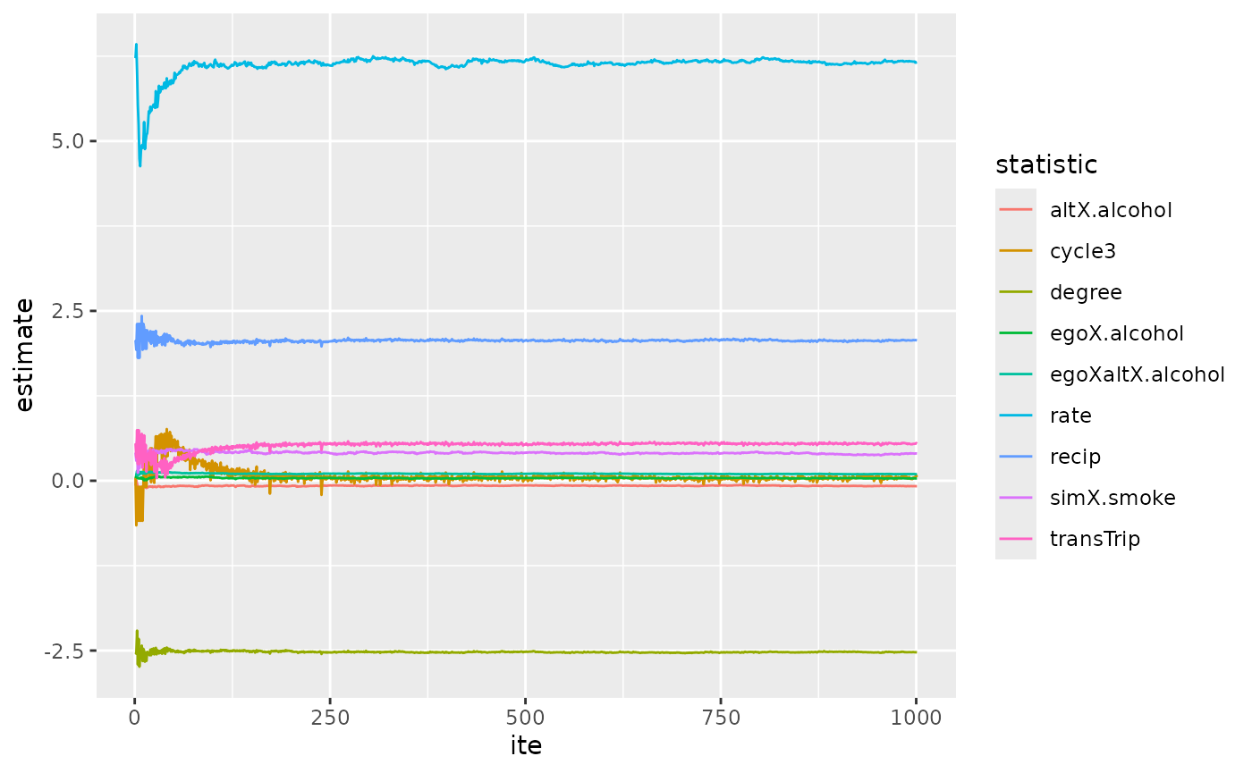

Let us zoom in a little on transTrip

df <- data.frame(ts_ans1c)
vars <- colnames(df)
df$ite <- 1:nrow(ts_ans1c)
#convert data from wide to long format
df <- df %>% pivot_longer(cols= vars[c(4)],
                          names_to='statistic',
                          values_to='estimate')

ggplot(df, aes(x=ite, y=estimate)) + 
  geom_line(aes(color=statistic))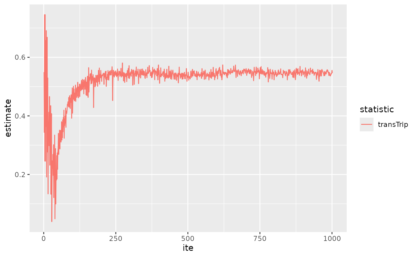

And on the last 250 iterations or so.

df <- data.frame(ts_ans1c)
vars <- colnames(df)
df$ite <- 1:nrow(ts_ans1c)
#convert data from wide to long format
df <- df[750:1000,] %>% pivot_longer(cols= vars[c(4)],
                          names_to='statistic',
                          values_to='estimate')

ggplot(df, aes(x=ite, y=estimate)) + 
  geom_line(aes(color=statistic))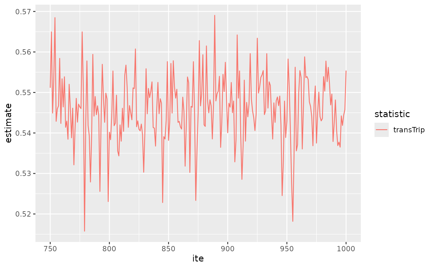

Well, what do you make out of this? If the lines keep oscillating around a specific value, try to increase the b parameter. Conversely, if the lines did not converge but you see no oscillation you could decrease the b parameter. In this case, I think we should/could increase b each 250 iterations or so.

You could also try to re-estimate the model with different starting values.

I like to inspect the results of the Robbins Monro algorithm in this way, before I go to phase3 because phase3 takes up quite some time.

4.3.3. Estimate SE, tstats and tconv.max

ESTIM <- ts_ans1c[nrow(ts_ans1c),] #we will take the last for now. 
ESTIM <- ans3$theta

ans1c_phase3 <- ts_phase3(startvalues = ESTIM, net1 = s501, net2= s502, statistics = STATS, ccovar = DF, itef3 = 1000, parallel = TRUE, returnDeps = TRUE, verbose = TRUE)

4.4 final results

Let us have a look at the final results.

SE <- sqrt(diag(ans1c_phase3$covtheta))
tstat <- ans1c_phase3$tstat
tconv.max <- ans1c_phase3$tconv.max
df <- data.frame(estim = ESTIM, SE = SE, "tratio" = tstat)

knitr::kable(df, digits = 3, "html", escape=FALSE, col.names = c("Estimate", "Standard <br> Error", "Convergence <br> t-ratio")) %>%
        kableExtra::kable_styling(bootstrap_options = c("striped", "hover")) %>%
        kableExtra::scroll_box(width = "100%", height = "500px") %>%
        kableExtra::footnote(general = paste("tconv.max:", round(tconv.max, 3), sep=" "))

	Estimate	Standard Error	Convergence t-ratio
Rate	6.230	0.963	0.016
degree	-2.521	0.138	0.074
recip	2.046	0.243	0.099
transTrip	0.543	0.150	0.097
cycle3	0.058	0.423	0.103
simX smoke	0.412	0.321	0.132
altX alcohol	-0.069	0.108	-0.093
egoX alcohol	0.038	0.094	-0.114
egoXaltX alcohol	0.099	0.074	-0.030
Note:
tconv.max: 0.185

My conclusion is that with RSienatwostep we can properly estimate a (very simple) network evolution model using the common ministep assumption. Good job!

5. Compare the estimates of the different twostep models

With different models I mean models with the same statistics but using different assumptions with respect to the theory of (inter)action.

I also think this is a nice workflow if we want to test robustness of ministep model:

estimate ministep model (with SE, and fit statistics)
estimate twostep models (phase2 only)
1. simultaneity
2. strict coordination
3. weak coordination
4. simstep
visually check model convergence
see if twostep models lead to (substantially) different estimates
if so, estimate phase3 of these models (and fit statistics) and compare final models
Compare GOF

5.1. estimate ministep model

We already did this above of course. But hey,..

5.1.1. via RSiena

#Step 1. prepare dataset
mynet <- sienaDependent(array(c(s501, s502), dim=c(50, 50, 2)))
alcohol <- s50a
smoke <- s50s
smoke <- coCovar(smoke[, 1])
alcohol <- coCovar(alcohol[, 1])
mydata <- sienaDataCreate(mynet, smoke, alcohol)

# Step 2. algorithm
myalgorithm <- sienaAlgorithmCreate(cond = FALSE, findiff = TRUE, projname=NULL) 

# Step 3. Define the model
myeff <- getEffects(mydata)
myeff <- includeEffects(myeff, cycle3, transTrip)
myeff <- includeEffects(myeff, egoX, altX, egoXaltX, interaction1 = "alcohol")
myeff <- includeEffects(myeff, simX, interaction1 = "smoke")

# Step 4. Estimate the model. 
ans3 <- siena07(myalgorithm, data=mydata, effects=myeff, batch=TRUE, returnDeps = TRUE)

5.1.2. via RsienaTwoStep

#Step 1. prepare dataset
DF <- data.frame(alcohol = s50a[, 1], smoke = s50s[, 1])
#Step 2. define the model 
STATS <- list(ts_degree, 
              ts_recip, 
              ts_transTrip, 
              ts_cycle3, 
              list(ts_simX, "smoke"), 
              list(ts_altX, "alcohol"), 
              list(ts_egoX, "alcohol"), 
              list(ts_egoXaltX, "alcohol"))
#Step 3. estimate Ministep model (default)
ts_ansMS <- ts_estim(net1 = s501, net2= s502, statistics = STATS, ccovar = DF, parallel = TRUE)

5.2. Estimate twostep models

5.2.1. phase2

We will use the ans of ’RSiena07()` as our input. We only estimate phase2. The goal is not so much to come to a perfect estimate but to check if the estimates are within the CI of the original estimates of RSiena. Only if this would not be the case, there may be a need to estimate the model by using different assumptions.

### simultaneity
ts_ansS <- ts_estim(ans = ans3, nite = 250, conv = 0.01, parallel = TRUE, phase3 = FALSE, p2step = c(0,1,0))
fsave(ts_ansS, "ts_ansS.rda")

### weak coordination
ts_ansWC <- ts_estim(ans = ans3, nite = 250, conv = 0.01, parallel = TRUE, phase3 = FALSE, p2step = c(0,1,0), dist1 = 2, dist2 = 2, modet1 = "degree", modet2 = "degree")
fsave(ts_ansWC, "ts_ansWC.rda")

### strict coordination
ts_ansSC <- ts_estim(ans = ans3, nite = 250, conv = 0.01, parallel = TRUE, phase3 = FALSE, p2step = c(0,1,0), dist1 = 2, modet1 = "degree" )
fsave(ts_ansSC, "ts_ansSC.rda")

### simstep
ts_ansST <- ts_estim(ans = ans3, nite = 250, conv = 0.01, parallel = TRUE, phase3 = FALSE, p2step = c(0,0,1))
fsave(ts_ansST, "ts_ansST.rda")

5.3. check convergence visually

We see that weak coordination, strict coordination and simstep stopped after the maximum of 250 iterations. Thus, for these models it takes (a bit) longer to reach convergence. We also observe more wobbly lines. But all in all, not too bad?

5.3.1. simultaneity

ts_ans <- ts_ansS
df <- data.frame(ts_ans)
vars <- colnames(df)
df$ite <- 1:nrow(ts_ans)
#convert data from wide to long format
df <- df %>% pivot_longer(cols= vars,
                          names_to='statistic',
                          values_to='estimate')

ggplot(df, aes(x=ite, y=estimate)) + 
  geom_line(aes(color=statistic))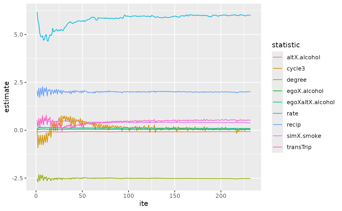

### 5.3.2. weak coordination

ts_ans <- ts_ansWC
df <- data.frame(ts_ans)
vars <- colnames(df)
df$ite <- 1:nrow(ts_ans)
#convert data from wide to long format
df <- df %>% pivot_longer(cols= vars,
                          names_to='statistic',
                          values_to='estimate')

ggplot(df, aes(x=ite, y=estimate)) + 
  geom_line(aes(color=statistic))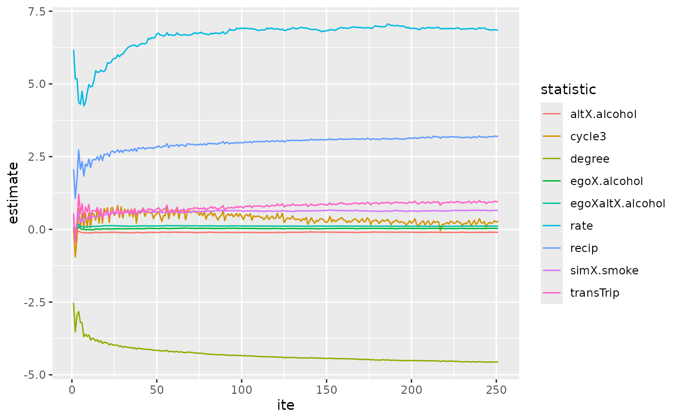

### 5.3.3. strict coordination

ts_ans <- ts_ansSC
df <- data.frame(ts_ans)
vars <- colnames(df)
df$ite <- 1:nrow(ts_ans)
#convert data from wide to long format
df <- df %>% pivot_longer(cols= vars,
                          names_to='statistic',
                          values_to='estimate')

ggplot(df, aes(x=ite, y=estimate)) + 
  geom_line(aes(color=statistic))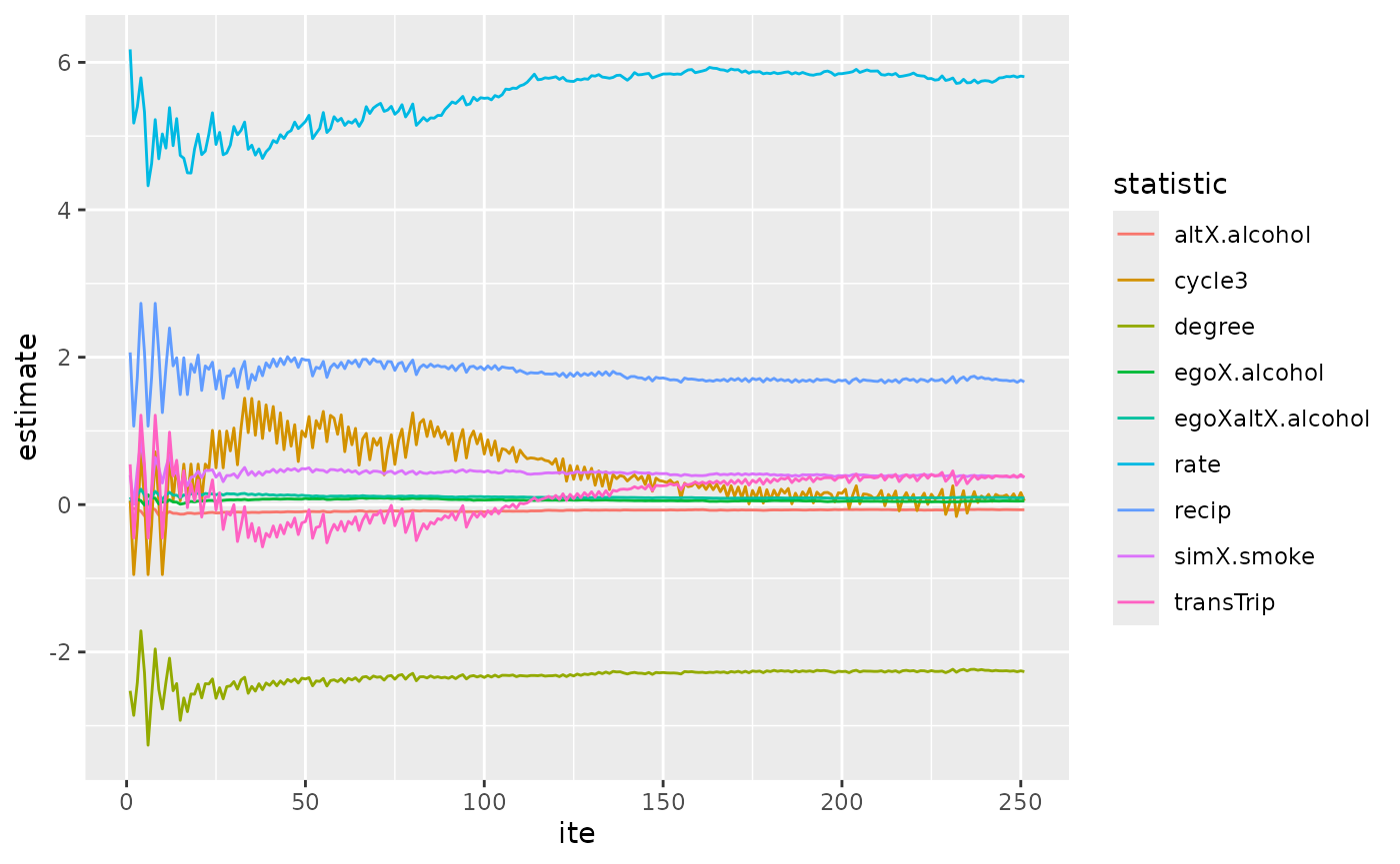

### 5.3.4. simstep

ts_ans <- ts_ansST
df <- data.frame(ts_ans)
vars <- colnames(df)
df$ite <- 1:nrow(ts_ans)
#convert data from wide to long format
df <- df %>% pivot_longer(cols= vars,
                          names_to='statistic',
                          values_to='estimate')

ggplot(df, aes(x=ite, y=estimate)) + 
  geom_line(aes(color=statistic))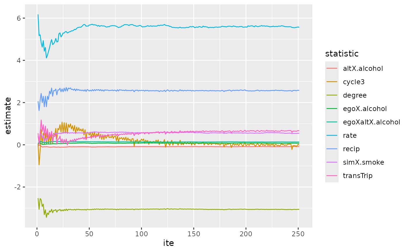

5.4. Compare estimates

#CI of RSiena
down <- ans3$theta - 1.96 * sqrt(diag(ans3$covtheta))
up <- ans3$theta + 1.96 * sqrt(diag(ans3$covtheta))

#our statistics
stats <-  factor(vars, levels = vars)
#final estimates 
b_s <- ts_ansS[nrow(ts_ansS),]
b_sc <- ts_ansSC[nrow(ts_ansSC),]
b_wc <- ts_ansWC[nrow(ts_ansWC),]
b_st <- ts_ansST[nrow(ts_ansST),]

#put everything in a dataframe
my.dt <- data.frame(statistics = stats, estimate=ans3$theta, down=down, up=up, b_s=b_s, b_sc=b_sc, b_wc=b_wc, b_st=b_st)

#use different layers to plot the separate estimates. and include a manual legend. 
ggplot(my.dt, aes(x=statistics, y=estimate)) +         
      geom_point(size = 3, aes(color="ministep")) +
      geom_errorbar(aes(ymin = down, ymax = up, color="ministep")) + 
      geom_point(size = 3, alpha = 0.5, aes(x=stats, y=b_s, color="simultaneity" )) + 
      geom_point(size = 3, alpha = 0.5, aes(x=stats, y=b_sc , color="strict coordination")) + 
  geom_point(size = 3, alpha = 0.5, aes(x=stats, y=b_wc, color="weak coordination")) + 
  geom_point(size = 3, alpha = 0.5, aes(x=stats, y=b_st, color="simstep")) + 
  scale_color_manual(name= "Estimation type", 
                     breaks = c("ministep", "simultaneity", "strict coordination", "weak coordination", "simstep"),
                     values = c("ministep"= "black", "simultaneity" = "red", "strict coordination" = "blue", "weak coordination" = "green", "simstep" = "orange")) + 
  scale_x_discrete(guide = guide_axis(n.dodge = 2)) +
  scale_y_continuous(n.breaks=10)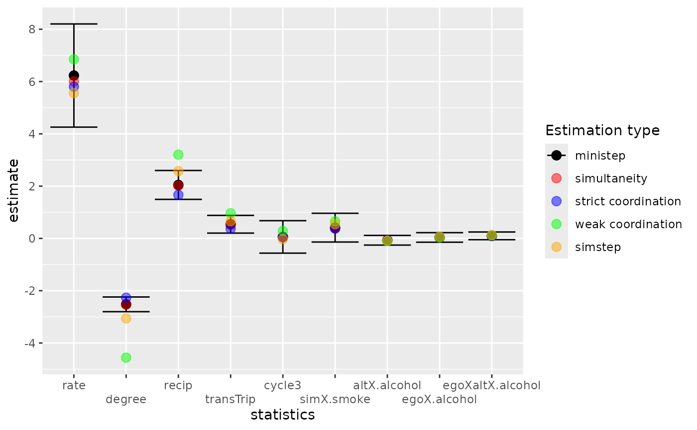

This figure already tells us that our twostep model more or less leads to similar estimates. There are some notably exceptions, however.

Weak coordination: much smaller degree estimate, much larger reciprocity estimate and larger transTrip estimate. This is not that strange since that under weak coordination the two alters have to be connected either at the beginning of the twostep or after the twostep.

5.5. phase3 for all twostep models

Please note, this can take a long time (more than a week), even with the relatively low itef3 default value of 100 in ts_phase3().

b_s <- ts_ansS[nrow(ts_ansS),]
b_sc <- ts_ansSC[nrow(ts_ansSC),]
b_wc <- ts_ansWC[nrow(ts_ansWC),]
b_st <- ts_ansST[nrow(ts_ansST),]

### simultaneity
ts_ansSp3 <- ts_phase3(mydata = mydata, myeff = myeff, startvalues =  b_s, parallel = TRUE, returnDeps = TRUE, p2step = c(0,1,0))
fsave(ts_ansSp3, "ts_ansSp3.rda")

### weak coordination
ts_ansWCp3 <- ts_phase3(mydata = mydata, myeff = myeff, startvalues =  b_wc, parallel = TRUE, returnDeps = TRUE, p2step = c(0,1,0), dist1 = 2, dist2 = 2, modet1 = "degree", modet2 = "degree")
fsave(ts_ansWCp3, "ts_ansWCp3.rda")

### strict coordination
ts_ansSCp3 <- ts_phase3(mydata = mydata, myeff = myeff, startvalues =  b_sc, parallel = TRUE, returnDeps = TRUE, p2step = c(0,1,0), dist1 = 2, modet1 = "degree")
fsave(ts_ansSCp3, "ts_ansSCp3.rda")

### simstep
ts_ansSTp3 <- ts_phase3(mydata = mydata, myeff = myeff, startvalues =  b_st, parallel = TRUE, returnDeps = TRUE, p2step = c(0,0,1))
fsave(ts_ansSTp3, "ts_ansSTp3.rda")

5.5.1 final results!

We conclude that all five different theories of interaction lead to similar conclusions with respect to significance of included statistics.

estim_MS <- ans3$theta
SE_MS <- sqrt(diag(ans3$covtheta))
tstat_MS <- ans3$tconv
tconv.max_MS <- ans3$tconv.max

estim_S <- ts_ansSp3$estim
SE_S <- sqrt(diag(ts_ansSp3$covtheta))
tstat_S <- ts_ansSp3$tstat
tconv.max_S <- ts_ansSp3$tconv.max

estim_WC <- ts_ansWCp3$estim
SE_WC <- sqrt(diag(ts_ansWCp3$covtheta))
tstat_WC <- ts_ansWCp3$tstat
tconv.max_WC <- ts_ansWCp3$tconv.max

estim_SC <- ts_ansSCp3$estim
SE_SC <- sqrt(diag(ts_ansSCp3$covtheta))
tstat_SC <- ts_ansSCp3$tstat
tconv.max_SC <- ts_ansSCp3$tconv.max

estim_ST <- ts_ansSTp3$estim
SE_ST <- sqrt(diag(ts_ansSTp3$covtheta))
tstat_ST <- ts_ansSTp3$tstat
tconv.max_ST <- ts_ansSTp3$tconv.max


df <- data.frame(estim_MS = estim_MS, SE_MS = SE_MS, tstat_MS = tstat_MS,
                estim_S = estim_S, SE_S = SE_S, tstat_S = tstat_S,
                 estim_WC = estim_WC, SE_WC = SE_WC, tstat_WC = tstat_WC,
                 estim_SC = estim_SC, SE_SC = SE_SC, tstat_SC = tstat_SC,
                 estim_ST = estim_ST, SE_ST = SE_ST, tstat_ST = tstat_ST)

results <- knitr::kable(df, digits = 3, "html",
             col.names = rep(c("Estim", "SE", "tstat"), 5)) %>% 
        kableExtra::add_header_above(c(" ", "ministep$^a$" = 3, "simultaneity$^b$" = 3, "weak coordination$^c$" = 3, "strict coordination$^d$" = 3, "simstep$^e$" = 3)) %>%
        kableExtra::kable_styling(bootstrap_options = c("striped", "hover")) %>%
  kableExtra::add_footnote(c(paste("tconv.max:", round(tconv.max_MS, 3), sep=" "),
                             paste("tconv.max:", round(tconv.max_S, 3), sep=" "),
                             paste("tconv.max:", round(tconv.max_WC, 3), sep=" "),
                             paste("tconv.max:", round(tconv.max_SC, 3), sep=" "),
                             paste("tconv.max:", round(tconv.max_ST, 3), sep=" ")
                             ), notation="alphabet") %>%
        kableExtra::scroll_box(width = "100%", height = "500px") 
        
results

	ministep\(^a\)			simultaneity\(^b\)			weak coordination\(^c\)			strict coordination\(^d\)			simstep\(^e\)
	Estim	SE	tstat	Estim	SE	tstat	Estim	SE	tstat	Estim	SE	tstat	Estim	SE	tstat
rate	6.230	1.007	0.045	6.002	0.923	-0.062	6.852	1.284	-0.003	5.805	0.941	-0.339	5.560	0.875	-0.126
degree	-2.521	0.143	0.017	-2.523	0.124	-0.092	-4.560	0.725	0.551	-2.266	0.124	-0.717	-3.058	0.215	-0.235
recip	2.046	0.282	-0.004	2.014	0.252	-0.097	3.205	0.567	0.466	1.666	0.265	-0.717	2.575	0.395	-0.233
transTrip	0.543	0.173	0.005	0.525	0.136	-0.125	0.963	0.285	0.354	0.369	0.116	-1.015	0.659	0.135	-0.256
cycle3	0.058	0.316	0.010	0.049	0.297	-0.114	0.285	0.598	0.373	0.052	0.256	-0.986	-0.027	0.439	-0.247
simX smoke	0.412	0.281	-0.014	0.387	0.365	-0.113	0.655	0.477	0.128	0.375	0.277	-0.362	0.544	0.395	-0.117
altX alcohol	-0.069	0.094	0.043	-0.069	0.105	0.153	-0.100	0.134	0.149	-0.070	0.094	0.041	-0.086	0.121	0.015
egoX alcohol	0.038	0.093	0.049	0.044	0.108	0.131	0.034	0.141	0.108	0.049	0.079	0.021	0.074	0.128	0.026
egoXaltX alcohol	0.099	0.075	-0.007	0.098	0.077	-0.118	0.113	0.112	0.341	0.090	0.064	-0.222	0.134	0.089	-0.071
^a tconv.max: 0.098
^b tconv.max: 0.251
^c tconv.max: 0.746
^d tconv.max: 1.072
^e tconv.max: 0.282

#kableExtra::save_kable(results, "./data/processed/results.html")

5.6. GOF

Overal conclusion:

for this data and this model specification (i.e. included statistics)
- ministep and simultaneity are more or less identical
- differences between the different theories of interaction are small
- simstep seems to be the best overal performance

5.6.1 GOF - degree distribution

df_tsMS <- ts_degreecount(sims=ans1c_phase3$simnets, simtype="ministep") 
df_tsS <- ts_degreecount(sims=ts_ansSp3$simnets, simtype="simultaneity") 
df_tsWC <- ts_degreecount(sims=ts_ansWCp3$simnets, simtype="weak coordination") 
df_tsSC <- ts_degreecount(sims=ts_ansSCp3$simnets, simtype="strict coordination") 
df_tsST <- ts_degreecount(sims=ts_ansSTp3$simnets, simtype="simstep") 

#targets
df_target <- ts_degreecount(list(s502), simtype="target")
df_target <- df_target[,c("x", "y")]
names(df_target)[2] <- "target"

df <- rbind(df_tsMS, df_tsS, df_tsWC, df_tsSC, df_tsST)
df <- left_join(df, df_target)
#focus in degree until 6
df_sel <- df[df$x=="deg1" | df$x=="deg2" | df$x=="deg3"| df$x=="deg4"| df$x=="deg5"| df$x=="deg6",]

p <- ggplot(df_sel, aes(x=x, y=y, fill=factor(type, levels=c("ministep", "simultaneity", "weak coordination", "strict coordination", "simstep"))) ) + 
  geom_violin(position=position_dodge(.8)) + 
  stat_summary( aes(x=x, y=target, fill=factor(type, levels=c("ministep", "simultaneity", "weak coordination", "strict coordination", "simstep"))), fun = mean,
               geom = "point",
               color="black", shape=10, position=position_dodge(.8)) + 
  stat_summary(fun = mean,
               geom = "errorbar",
               fun.max = function(x) mean(x) + sd(x),
               fun.min = function(x) mean(x) - sd(x),
               width=.1,
               color="red", position=position_dodge(.8)) + 
  stat_summary(fun = mean,
               geom = "point",
               color="red", position=position_dodge(.8)) + 
  labs(x = "degree", y = "degree count", fill="simulation type") 
  

p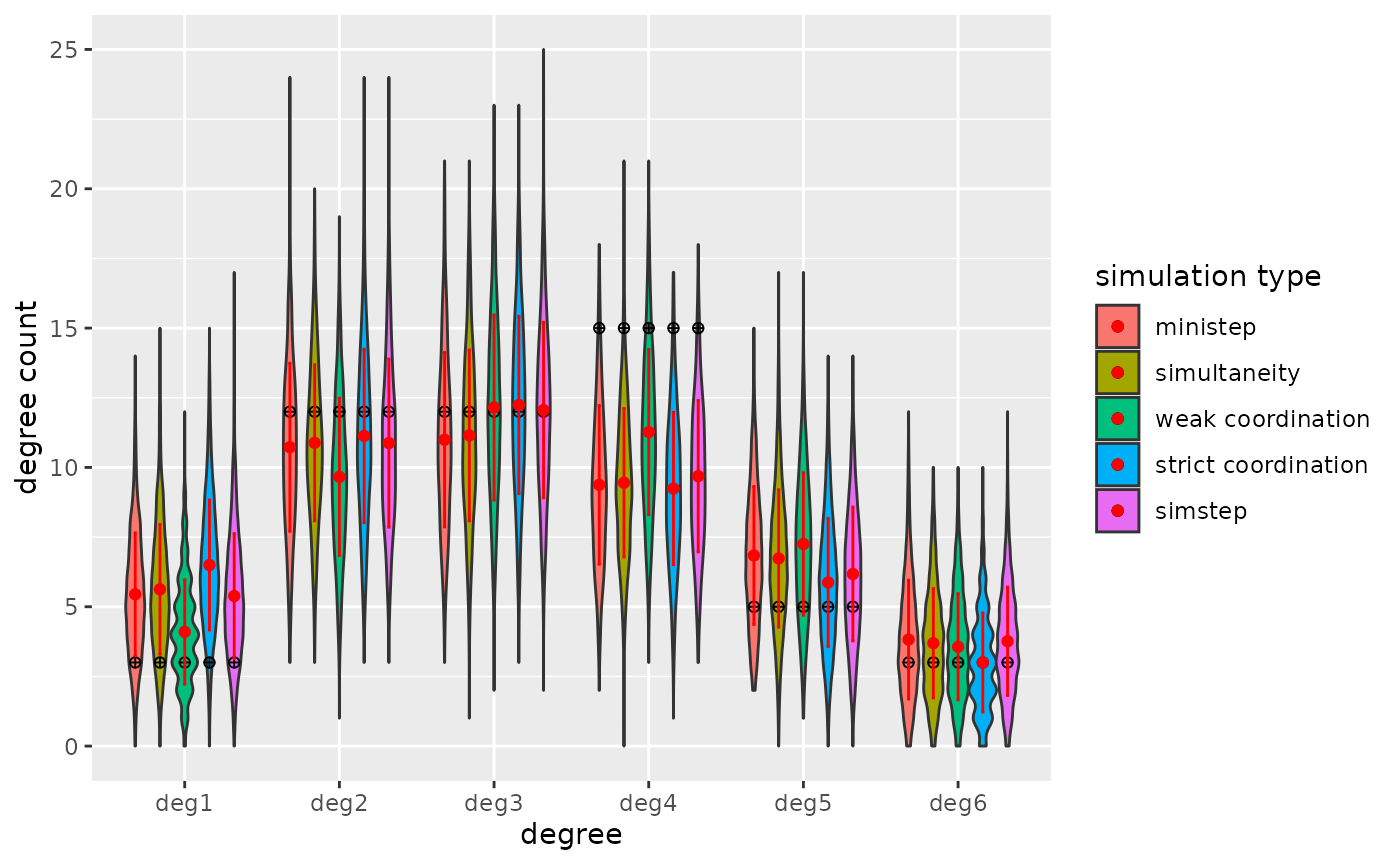

Interesting!!

Some tentative conclusions:

no difference between simultaneity and ministep
weak coordination is best for degree 1 and degree 4. At higher degrees (5 and 6) is strict coordination the best.
simstep is either just as good as ministep or outperforms ministep

5.6.2. GOF - dyad census

df_tsMS <- ts_dyads(sims=ans1c_phase3$simnets, simtype="ministep") 
df_tsS <- ts_dyads(sims=ts_ansSp3$simnets, simtype="simultaneity") 
df_tsWC <- ts_dyads(sims=ts_ansWCp3$simnets, simtype="weak coordination") 
df_tsSC <- ts_dyads(sims=ts_ansSCp3$simnets, simtype="strict coordination") 
df_tsST <- ts_dyads(sims=ts_ansSTp3$simnets, simtype="simstep") 

#targets
df_target <- ts_dyads(list(s502), simtype="target")
df_target <- df_target[,c("x", "y")]
names(df_target)[2] <- "target"

df <- rbind(df_tsMS, df_tsS, df_tsWC, df_tsSC, df_tsST)
df <- left_join(df, df_target)

df_sel <- df[df$x=="asym" | df$x=="mut" ,]

p <- ggplot(df_sel, aes(x=x, y=y, fill=factor(type, levels=c("ministep", "simultaneity", "weak coordination", "strict coordination", "simstep"))) ) + 
  geom_violin(position=position_dodge(.8)) + 
  stat_summary(fun = mean,
               geom = "errorbar",
               fun.max = function(x) mean(x) + sd(x),
               fun.min = function(x) mean(x) - sd(x),
               width=.1,
               color="red", position=position_dodge(.8)) + 
  stat_summary(fun = mean,
               geom = "point",
               color="red", position=position_dodge(.8)) + 
  stat_summary( aes(x=x, y=target, fill=factor(type, levels=c("ministep", "simultaneity", "weak coordination", "strict coordination", "simstep"))), fun = mean,
               geom = "point",
               color="black", shape=10, position=position_dodge(.8)) +
  labs(x = "dyad type", y = "dyad count", fill="simulation type")

p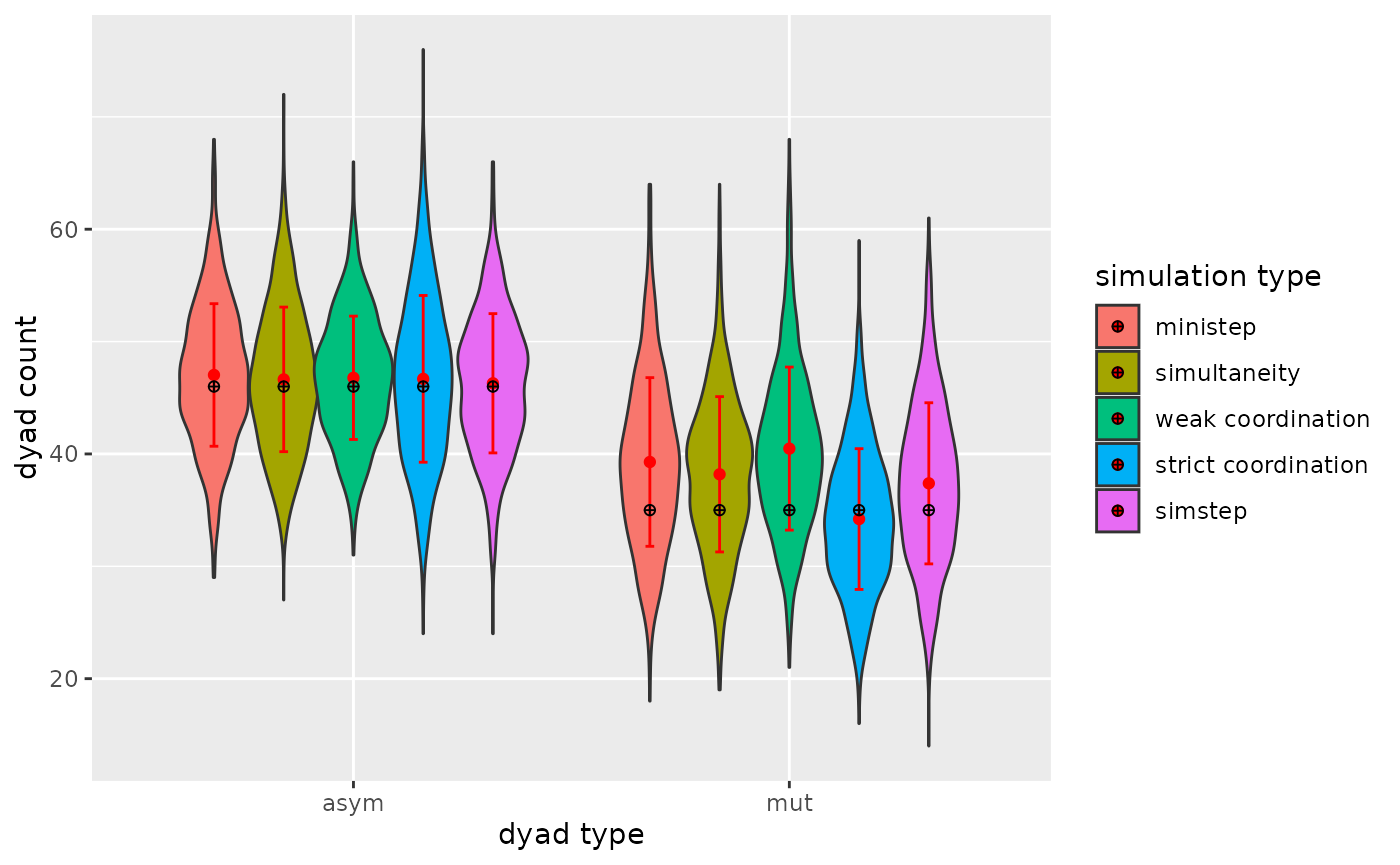

Conclusion:

strict coordination seems to be the winner.
simstep is outperforming ministep.

5.6.3. GOF - triad census

df_tsMS <- ts_triads(sims=ans1c_phase3$simnets, simtype="ministep") 
df_tsS <- ts_triads(sims=ts_ansSp3$simnets, simtype="simultaneity") 
df_tsWC <- ts_triads(sims=ts_ansWCp3$simnets, simtype="weak coordination") 
df_tsSC <- ts_triads(sims=ts_ansSCp3$simnets, simtype="strict coordination") 
df_tsST <- ts_triads(sims=ts_ansSTp3$simnets, simtype="simstep") 

#targets
df_target <- ts_triads(list(s502), simtype="target")
df_target <- df_target[,c("x", "y")]
names(df_target)[2] <- "target"

df <- rbind(df_tsMS, df_tsS, df_tsWC, df_tsSC, df_tsST)
df <- left_join(df, df_target)
#> Joining with `by = join_by(x)`

df_sel <- df[df$x=="021D" | df$x=="021U" | df$x=="021C",]

p <- ggplot(df_sel, aes(x=x, y=y, fill=factor(type, levels=c("ministep", "simultaneity", "weak coordination", "strict coordination", "simstep"))) ) + 
  geom_violin(position=position_dodge(.8)) + 
  stat_summary(fun = mean,
               geom = "errorbar",
               fun.max = function(x) mean(x) + sd(x),
               fun.min = function(x) mean(x) - sd(x),
               width=.1,
               color="red", position=position_dodge(.8)) + 
  stat_summary(fun = mean,
               geom = "point",
               color="red", position=position_dodge(.8)) + 
  stat_summary( aes(x=x, y=target, fill=factor(type, levels=c("ministep", "simultaneity", "weak coordination", "strict coordination", "simstep"))), fun = mean,
               geom = "point",
               color="black", shape=10, position=position_dodge(.8)) +
  labs(x = "triad type", y = "triad count", fill="simulation type")

p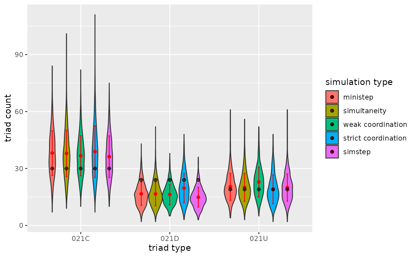

Conclusion:

strict coordination seems to be the winner.
simstep is not outperforming ministep for triad configurations.

5.6.4. GOF - smoke segregation

df_tsMS <- ts_nacf(sims=ans1c_phase3$simnets, simtype="ministep", cov=DF$smoke) 
df_tsS <- ts_nacf(sims=ts_ansSp3$simnets, simtype="simultaneity", cov=DF$smoke) 
df_tsWC <- ts_nacf(sims=ts_ansWCp3$simnets, simtype="weak coordination", cov=DF$smoke) 
df_tsSC <- ts_nacf(sims=ts_ansSCp3$simnets, simtype="strict coordination", cov=DF$smoke) 
df_tsST <- ts_nacf(sims=ts_ansSTp3$simnets, simtype="simstep", cov=DF$smoke) 

#targets
df_target <- ts_nacf(list(s502), simtype="target", cov=DF$smoke)
names(df_target)[1] <- "target"

df <- rbind(df_tsMS, df_tsS, df_tsWC, df_tsSC, df_tsST)
names(df)[1] <- "MoranI" 
df$target <- df_target$target

p <- ggplot(df, aes(x=factor(type, levels=c("ministep", "simultaneity", "weak coordination", "strict coordination", "simstep")), y=MoranI, fill=factor(type, levels=c("ministep", "simultaneity", "weak coordination", "strict coordination", "simstep"))) ) + 
  geom_violin(position=position_dodge(.8)) + 
  stat_summary(fun = mean,
               geom = "errorbar",
               fun.max = function(x) mean(x) + sd(x),
               fun.min = function(x) mean(x) - sd(x),
               width=.1,
               color="red", position=position_dodge(.8)) + 
  stat_summary(fun = mean,
               geom = "point",
               color="red", position=position_dodge(.8)) + 
  stat_summary( aes(x=factor(type, levels=c("ministep", "simultaneity", "weak coordination", "strict coordination", "simstep")), y=target, fill=factor(type, levels=c("ministep", "simultaneity", "weak coordination", "strict coordination", "simstep"))), fun = mean,
               geom = "point",
               color="black", shape=10, position=position_dodge(.8)) +
  labs(x = "simulation type", y = "smoke segregation (MoranI)", fill="simulation type") +
  scale_x_discrete(guide = guide_axis(n.dodge = 2))

p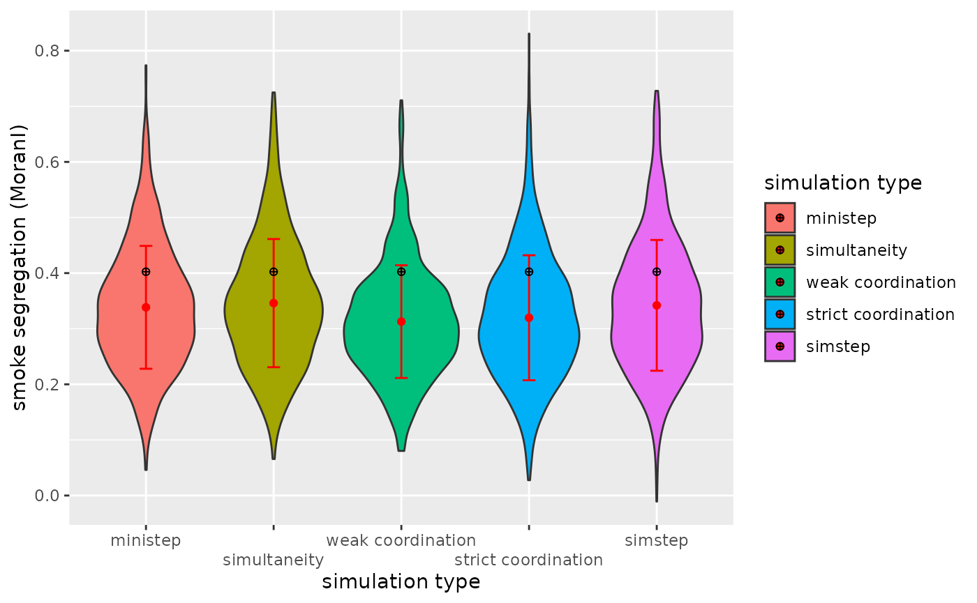

Conclusion:

weak and strict coordination are doing worst

6. Conclusion

RsienaTwoStep offers a workflow for assessing the extent to which the ministep assumption is crucial. By crucial I mean that parameter estimates and model fit depend on the chosen ‘micro theory of interaction’.
In the above example, the assumption is not crucial. All theories of interaction lead to similar conclusions with respect to the significance of the included statistics and the GOF of the ministep and twostep models are very similar. Perhaps the simstep models has the best GOF.

1. Getting started

1.1. Basic functions

1.2. Packages

2. Setting up cluster

3. Running Siena07()

3.1. Prepare the dataset

3.2. Set up up the algorithm.

3.3. Define the model

3.4. Estimate the model.

4. Estimate via RsienaTwoStep

4.1. Prepare the dataset

4.2. Define the model.

4.2.1. Check statistics

4.3. Estimate model

4.3.1. Estimate parameters.

4.3.2. check convergence visually

4.3.3. Estimate SE, tstats and tconv.max

4.4 final results

5. Compare the estimates of the different twostep models

5.1. estimate ministep model

5.1.1. via RSiena

5.1.2. via RsienaTwoStep

5.2. Estimate twostep models

5.2.1. phase2

5.3. check convergence visually

5.3.1. simultaneity

5.4. Compare estimates

5.5. phase3 for all twostep models

5.5.1 final results!

5.6. GOF

5.6.1 GOF - degree distribution

5.6.2. GOF - dyad census

5.6.3. GOF - triad census

5.6.4. GOF - smoke segregation

6. Conclusion

3. Running `Siena07()`

4. Estimate via `RsienaTwoStep`