Chapter 5 Methods
5.2 Consequences
In this part we we start with estimating a micro-macro model. See Figure 5.1 which I adapted from Bennink et al. (2016) for the basic idea. We have to realize that our data has a hierarchical structure: observations (confidants/ties) at the lowest-level (level-one, micro-level, tie-level or confidant-level) are nested in a higher level (level-two, macro-level, network-level or ego-level) and that these observations at the confidant-level are interdependent. We need to take these interdependencies into account.
Moreover, if we wish to relate characteristics of our CDN to characteristics of our egos - and yes that is our wish in this section -, our dependent variable is at the macro-level and we ‘have to’ estimate a micro-macro model. Please read Croon and Veldhoven (2007) and Bennink et al. (2016).9
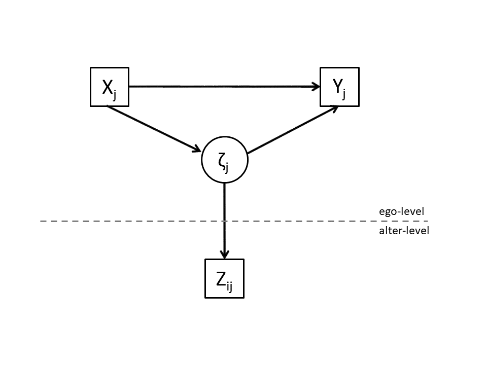
Figure 5.1: Basic micro-macro model
note: Adapted from Bennink et al. (2016)
In chapter 3 we investigated how spouses influence each others political opinion. In this chapter we continue our discussion but now with respect to our confidants. Suppose we want to investigate how our confidants influence our political opinions. Unfortunately, not many surveys that map the Core Discussion Network include name interpreter questions on the political opinions of the named confidants. However, one of the most important determinant for someone’s political opinion is his/her educational attainment.
There are several theoretical reasons why the educational attainment of our confidants would impact our own opinions. To mention just a few:
- Education of alter is ‘a proxy’ of alter’s opinions and alter’s opinions may influence our opinions.
- Alters with different educational levels have different life experiences and the life experiences of our alters may influence our opinions.
- Alters with different educational levels have different knowledge on topics, sharing knowledge on these topics may influence our opinions.
5.3 Research questions
This leads to the following research question:
- To what extent does the educational level of our confidants influence our political opinions?
- To what extent does the impact of the educational level of our confidants on our political opinion depend on:
- ego characteristics (e.g. educational level)?
- characteristics of our Core Discussion Network as a whole (e.g size)?
- other characteristics of our confidants (e.g age or gender)?
For each ego (at each time point) we may have information on one to five confidants. As already stated above, these observations are interdependent and we need to take this into account. Naturally, we also need to be aware that our own educational-level (and political opinion) will influence with whom we discuss important matters. Thus, we need to take into account selection effects.
5.4 Data
We will use the data from the LISS panel.

More concretely, we will use:
- 11 waves (2008-2014, 2016-2019)
- Filter on respondents older than 25.
We have already constructed a dataset for you guys and gals to work with which contains information on more than 13000 respondents. Don’t forget it is a panel data set. This means we have more observations for the same respondent (and his/her CDN) over time.
Please download this data file to your working directory.
5.4.1 Variables
Variables of interest and value labels:
Ego-level:
- ego_id
- educ
- gender
- age
- eu: opinion of ego on eu_integration: 0 = eu integration has gone too far / 4 = eu
- eu_integration: 0 = eu integration has gone too far / 4 = eu integration should go further
- immigrants: 0 = immigrants should adjust / 4 immigrants can retain their own culture.
- euthanasia: 1 = euthanasia should be forbidden / 5 euthanasia should be permitted
- income_diff: 1 differences in income should increase / 5 differences in income should decrease
confidant-level:
- educ_alterx
- gender_alterx
- age_alterx
The x refers to the x-mentioned confidant (1-5).
In the wide dataset each variable ends with “.y” where .y refers to the survey wave. Thus educ_alter4.9 refers to the educational level in years of the fourth mentioned confidant in survey_wave 9 (i.e. 2017).
For the original variables in Dutch see below:
EU integratie
De Europese integratie is te ver gegaan.
1 Helemaal oneens
2 Oneens
3 Niet eens, niet oneens
4 Eens
5 Helemaal eens
opleiding
Hoogste opleiding met diploma
1 basisonderwijs
2 vmbo
3 havo/vwo
4 mbo
5 hbo
6 wo
7 anders
8 (Nog) geen onderwijs afgerond
9 Volgt nog geen onderwijs
Hierbij hebben wij opleiding gecategoriseerd in drie groepen:
1. Laag: basisonderwijs en vmbo
2. Midden: havo/vwo en mbo
3. Hoog: hbo en wo
We nemen enkel mensen van 25 jaar en ouder mee. Van hen verwachten we dat ze klaar zijn met hun onderwijscarriere.
5.4.2 Preperation
#### clean the environment ####.
rm(list = ls())

#### packages ####.
require(tidyverse)
require(lavaan)

##### Data input ###.
load("addfiles/liss_cdn.Rdata")

liss_l <- liss_cdn[[1]]
liss_w <- liss_cdn[[2]]
Let us for now focus on the last wave. Thus wave 2019 (wave 11).
In the literature two approaches are discussed to estimate a micro-macro model, a persons as variables approach and a multi-level approach. The persons as variables approach is - I hope - easiest to implement and for that we need the data in wide format (one row for each respondent). The idea is that the alter scores load on a latent variable at the ego-level. This latent variable has a random component at the ego-level (cf. random intercept in multi-level models). In a basic model with continous manifest variables at the micro-level, the latent variable at the macro-level is the (biased corrected) mean.
5.5 Disaggregation method
But first let us estimate the wrong models. We will start with a disaggregation approach. We need to disaggregate our data so that each row refers to a specific combination of ego, survey_wave and alter.
# we need to disaggregate our data. thus each ego, wave, alter per row.
liss_ll <- rbind(liss_l, liss_l, liss_l, liss_l, liss_l)
liss_ll$index_alter <- rep(1:5, each = length(liss_l[, 1]))
liss_ll$educ_alter <- NA

liss_ll$educ_alter <- ifelse(liss_ll$index_alter == 1, liss_ll$educ_alter1, liss_ll$educ_alter)
liss_ll$educ_alter <- ifelse(liss_ll$index_alter == 2, liss_ll$educ_alter2, liss_ll$educ_alter)
liss_ll$educ_alter <- ifelse(liss_ll$index_alter == 3, liss_ll$educ_alter3, liss_ll$educ_alter)
liss_ll$educ_alter <- ifelse(liss_ll$index_alter == 4, liss_ll$educ_alter4, liss_ll$educ_alter)
liss_ll$educ_alter <- ifelse(liss_ll$index_alter == 5, liss_ll$educ_alter5, liss_ll$educ_alter)

liss_ll_sel <- liss_ll %>%
    filter(survey_wave == 11)

model1 <- "
  euthanasia ~ educ_alter
  euthanasia ~ 1
  euthanasia ~~ euthanasia
  "


fit1 <- lavaan(model1, data = liss_ll_sel)
summary(fit1)
#> lavaan 0.6-11 ended normally after 15 iterations
#>
#> Estimator ML
#> Optimization method NLMINB
#> Number of model parameters 3
#>
#> Used Total
#> Number of observations 10923 29925
#>
#> Model Test User Model:
#>
#> Test statistic 0.000
#> Degrees of freedom 0
#>
#> Parameter Estimates:
#>
#> Standard errors Standard
#> Information Expected
#> Information saturated (h1) model Structured
#>
#> Regressions:
#> Estimate Std.Err z-value P(>|z|)
#> euthanasia ~
#> educ_alter 0.009 0.003 2.726 0.006
#>
#> Intercepts:
#> Estimate Std.Err z-value P(>|z|)
#> .euthanasia 4.335 0.042 102.363 0.000
#>
#> Variances:
#> Estimate Std.Err z-value P(>|z|)
#> .euthanasia 0.921 0.012 73.902 0.0005.6 Aggregation method
We could also try to aggregate our confidant data. This means we calculate the mean educational level of our confidants solely based on the available data in the observed scores.
liss_l <- liss_l %>%
    mutate(educ_alter_mean = rowMeans(cbind(educ_alter1, educ_alter2, educ_alter3, educ_alter4, educ_alter5),
        na.rm = TRUE))  #calculate the mean educational level of the alters.

liss_l_sel <- liss_l %>%
    filter(survey_wave == 11)

model1 <- "
  euthanasia ~ educ_alter_mean
  euthanasia ~ 1
  euthanasia ~~ euthanasia
  "

fit2 <- lavaan(model1, data = liss_l_sel, missing = "fiml")
summary(fit2)
#> lavaan 0.6-11 ended normally after 15 iterations
#>
#> Estimator ML
#> Optimization method NLMINB
#> Number of model parameters 3
#>
#> Used Total
#> Number of observations 3743 5985
#> Number of missing patterns 2
#>
#> Model Test User Model:
#>
#> Test statistic 0.000
#> Degrees of freedom 0
#>
#> Parameter Estimates:
#>
#> Standard errors Standard
#> Information Observed
#> Observed information based on Hessian
#>
#> Regressions:
#> Estimate Std.Err z-value P(>|z|)
#> euthanasia ~
#> educ_alter_men 0.016 0.008 2.020 0.043
#>
#> Intercepts:
#> Estimate Std.Err z-value P(>|z|)
#> .euthanasia 4.244 0.098 43.513 0.000
#>
#> Variances:
#> Estimate Std.Err z-value P(>|z|)
#> .euthanasia 0.934 0.023 41.207 0.0005.7 Micro-macro model
Finally, let us estimate a better model. We will not use the observed mean value of the educational levels of the confidants for each ego but will calculate a bias corrected mean.
liss_l_sel <- liss_l %>%
    filter(survey_wave == 11)

model <- "
  #latent variable
  FX =~ 1*educ_alter1
  FX =~ 1*educ_alter2
  FX =~ 1*educ_alter3
  FX =~ 1*educ_alter4
  FX =~ 1*educ_alter5

  #variances
  educ_alter1 ~~ b*educ_alter1
  educ_alter2 ~~ b*educ_alter2
  educ_alter3 ~~ b*educ_alter3
  educ_alter4 ~~ b*educ_alter4
  educ_alter5 ~~ b*educ_alter5


  FX ~~ FX
  euthanasia ~~ euthanasia

  #regression model
  euthanasia ~ FX
  euthanasia ~ 1

  #intercepts/means
  educ_alter1 ~ e*1
  educ_alter2 ~ e*1
  educ_alter3 ~ e*1
  educ_alter4 ~ e*1
  educ_alter5 ~ e*1
"


fit3 <- lavaan(model, data = liss_l_sel, missing = "fiml", fixed.x = FALSE)
summary(fit3)
#> lavaan 0.6-11 ended normally after 22 iterations
#>
#> Estimator ML
#> Optimization method NLMINB
#> Number of model parameters 14
#> Number of equality constraints 8
#>
#> Used Total
#> Number of observations 4922 5985
#> Number of missing patterns 50
#>
#> Model Test User Model:
#>
#> Test statistic 46.488
#> Degrees of freedom 21
#> P-value (Chi-square) 0.001
#>
#> Parameter Estimates:
#>
#> Standard errors Standard
#> Information Observed
#> Observed information based on Hessian
#>
#> Latent Variables:
#> Estimate Std.Err z-value P(>|z|)
#> FX =~
#> educ_alter1 1.000
#> educ_alter2 1.000
#> educ_alter3 1.000
#> educ_alter4 1.000
#> educ_alter5 1.000
#>
#> Regressions:
#> Estimate Std.Err z-value P(>|z|)
#> euthanasia ~
#> FX 0.032 0.015 2.083 0.037
#>
#> Intercepts:
#> Estimate Std.Err z-value P(>|z|)
#> .euthanasia 4.423 0.015 303.122 0.000
#> .educ_altr1 (e) 12.487 0.034 370.005 0.000
#> .educ_altr2 (e) 12.487 0.034 370.005 0.000
#> .educ_altr3 (e) 12.487 0.034 370.005 0.000
#> .educ_altr4 (e) 12.487 0.034 370.005 0.000
#> .educ_altr5 (e) 12.487 0.034 370.005 0.000
#> FX 0.000
#>
#> Variances:
#> Estimate Std.Err z-value P(>|z|)
#> .educ_altr1 (b) 5.438 0.083 65.318 0.000
#> .educ_altr2 (b) 5.438 0.083 65.318 0.000
#> .educ_altr3 (b) 5.438 0.083 65.318 0.000
#> .educ_altr4 (b) 5.438 0.083 65.318 0.000
#> .educ_altr5 (b) 5.438 0.083 65.318 0.000
#> FX 2.322 0.099 23.418 0.000
#> .euthanasia 0.972 0.020 47.642 0.0005.8 Random Intercept Cross-Lagged Micro-Macro Model RI-CLP-MM
Of course we want to take into account selection effects. That is, ego’s opinion may also affect the educational level of his/her confidants. Luckily, you are very familiar by now with the RI-CLPM (if not, see section 3.6.2. Let us try to combine the micro-macro model with a RI-CLPM (let’s call it an RI-CLP-MM).
To illustrate I only use four waves: 6-9.
5.8.1 Measurement model
We need to calculate the bias corrected means for each wave. I prefer to do that in a two-step procedure.
myModel <- '

FX6 =~ 1*educ_alter1.6 + 1*educ_alter2.6 + 1*educ_alter3.6 + 1*educ_alter4.6 + 1*educ_alter5.6
FX7 =~ 1*educ_alter1.7 + 1*educ_alter2.7 + 1*educ_alter3.7 + 1*educ_alter4.7 + 1*educ_alter5.7
FX8 =~ 1*educ_alter1.8 + 1*educ_alter2.8 + 1*educ_alter3.8 + 1*educ_alter4.8 + 1*educ_alter5.8
FX9 =~ 1*educ_alter1.9 + 1*educ_alter2.9 + 1*educ_alter3.9 + 1*educ_alter4.9 + 1*educ_alter5.9

#variances of latent variables
FX6 ~~ FX6
FX7 ~~ FX7
FX8 ~~ FX8
FX9 ~~ FX9

#constrained variances of manifest variables
educ_alter1.6 ~~ a*educ_alter1.6
educ_alter2.6 ~~ a*educ_alter2.6
educ_alter3.6 ~~ a*educ_alter3.6
educ_alter4.6 ~~ a*educ_alter4.6
educ_alter5.6 ~~ a*educ_alter5.6

educ_alter1.7 ~~ b*educ_alter1.7
educ_alter2.7 ~~ b*educ_alter2.7
educ_alter3.7 ~~ b*educ_alter3.7
educ_alter4.7 ~~ b*educ_alter4.7
educ_alter5.7 ~~ b*educ_alter5.7

educ_alter1.8 ~~ c*educ_alter1.8
educ_alter2.8 ~~ c*educ_alter2.8
educ_alter3.8 ~~ c*educ_alter3.8
educ_alter4.8 ~~ c*educ_alter4.8
educ_alter5.8 ~~ c*educ_alter5.8

educ_alter1.9 ~~ d*educ_alter1.9
educ_alter2.9 ~~ d*educ_alter2.9
educ_alter3.9 ~~ d*educ_alter3.9
educ_alter4.9 ~~ d*educ_alter4.9
educ_alter5.9 ~~ d*educ_alter5.9


#contrained intercepts of the manifest variables (structural changes are picked up by the latent variables)
educ_alter1.6 ~ e*1
educ_alter2.6 ~ e*1
educ_alter3.6 ~ e*1
educ_alter4.6 ~ e*1
educ_alter5.6 ~ e*1

educ_alter1.7 ~ e*1
educ_alter2.7 ~ e*1
educ_alter3.7 ~ e*1
educ_alter4.7 ~ e*1
educ_alter5.7 ~ e*1

educ_alter1.8 ~ e*1
educ_alter2.8 ~ e*1
educ_alter3.8 ~ e*1
educ_alter4.8 ~ e*1
educ_alter5.8 ~ e*1

educ_alter1.9 ~ e*1
educ_alter2.9 ~ e*1
educ_alter3.9 ~ e*1
educ_alter4.9 ~ e*1
educ_alter5.9 ~ e*1


#free the means of the latent variables

FX7 ~ 1
FX8 ~ 1
FX9 ~ 1
'

fit <- lavaan(myModel, data = liss_w, missing = 'ML', fixed.x=FALSE, meanstructure = T)
summary(fit, standardized = T)
#> lavaan 0.6-11 ended normally after 38 iterations
#>
#> Estimator ML
#> Optimization method NLMINB
#> Number of model parameters 47
#> Number of equality constraints 35
#>
#> Used Total
#> Number of observations 6582 13018
#> Number of missing patterns 1740
#>
#> Model Test User Model:
#>
#> Test statistic 13075.965
#> Degrees of freedom 218
#> P-value (Chi-square) 0.000
#>
#> Parameter Estimates:
#>
#> Standard errors Standard
#> Information Observed
#> Observed information based on Hessian
#>
#> Latent Variables:
#> Estimate Std.Err z-value P(>|z|) Std.lv Std.all
#> FX6 =~
#> educ_alter1.6 1.000 1.482 0.538
#> educ_alter2.6 1.000 1.482 0.538
#> educ_alter3.6 1.000 1.482 0.538
#> educ_alter4.6 1.000 1.482 0.538
#> educ_alter5.6 1.000 1.482 0.538
#> FX7 =~
#> educ_alter1.7 1.000 1.508 0.543
#> educ_alter2.7 1.000 1.508 0.543
#> educ_alter3.7 1.000 1.508 0.543
#> educ_alter4.7 1.000 1.508 0.543
#> educ_alter5.7 1.000 1.508 0.543
#> FX8 =~
#> educ_alter1.8 1.000 1.546 0.557
#> educ_alter2.8 1.000 1.546 0.557
#> educ_alter3.8 1.000 1.546 0.557
#> educ_alter4.8 1.000 1.546 0.557
#> educ_alter5.8 1.000 1.546 0.557
#> FX9 =~
#> educ_alter1.9 1.000 1.538 0.557
#> educ_alter2.9 1.000 1.538 0.557
#> educ_alter3.9 1.000 1.538 0.557
#> educ_alter4.9 1.000 1.538 0.557
#> educ_alter5.9 1.000 1.538 0.557
#>
#> Intercepts:
#> Estimate Std.Err z-value P(>|z|) Std.lv Std.all
#> .edc_ltr1.6 (e) 12.167 0.031 393.604 0.000 12.167 4.421
#> .edc_ltr2.6 (e) 12.167 0.031 393.604 0.000 12.167 4.421
#> .edc_ltr3.6 (e) 12.167 0.031 393.604 0.000 12.167 4.421
#> .edc_ltr4.6 (e) 12.167 0.031 393.604 0.000 12.167 4.421
#> .edc_ltr5.6 (e) 12.167 0.031 393.604 0.000 12.167 4.421
#> .edc_ltr1.7 (e) 12.167 0.031 393.604 0.000 12.167 4.386
#> .edc_ltr2.7 (e) 12.167 0.031 393.604 0.000 12.167 4.386
#> .edc_ltr3.7 (e) 12.167 0.031 393.604 0.000 12.167 4.386
#> .edc_ltr4.7 (e) 12.167 0.031 393.604 0.000 12.167 4.386
#> .edc_ltr5.7 (e) 12.167 0.031 393.604 0.000 12.167 4.386
#> .edc_ltr1.8 (e) 12.167 0.031 393.604 0.000 12.167 4.381
#> .edc_ltr2.8 (e) 12.167 0.031 393.604 0.000 12.167 4.381
#> .edc_ltr3.8 (e) 12.167 0.031 393.604 0.000 12.167 4.381
#> .edc_ltr4.8 (e) 12.167 0.031 393.604 0.000 12.167 4.381
#> .edc_ltr5.8 (e) 12.167 0.031 393.604 0.000 12.167 4.381
#> .edc_ltr1.9 (e) 12.167 0.031 393.604 0.000 12.167 4.406
#> .edc_ltr2.9 (e) 12.167 0.031 393.604 0.000 12.167 4.406
#> .edc_ltr3.9 (e) 12.167 0.031 393.604 0.000 12.167 4.406
#> .edc_ltr4.9 (e) 12.167 0.031 393.604 0.000 12.167 4.406
#> .edc_ltr5.9 (e) 12.167 0.031 393.604 0.000 12.167 4.406
#> FX7 0.057 0.043 1.343 0.179 0.038 0.038
#> FX8 0.199 0.044 4.472 0.000 0.129 0.129
#> FX9 0.248 0.045 5.520 0.000 0.161 0.161
#> FX6 0.000 0.000 0.000
#>
#> Variances:
#> Estimate Std.Err z-value P(>|z|) Std.lv Std.all
#> FX6 2.195 0.089 24.725 0.000 1.000 1.000
#> FX7 2.273 0.085 26.832 0.000 1.000 1.000
#> FX8 2.390 0.093 25.606 0.000 1.000 1.000
#> FX9 2.366 0.095 24.867 0.000 1.000 1.000
#> .edc_ltr1.6 (a) 5.378 0.077 70.264 0.000 5.378 0.710
#> .edc_ltr2.6 (a) 5.378 0.077 70.264 0.000 5.378 0.710
#> .edc_ltr3.6 (a) 5.378 0.077 70.264 0.000 5.378 0.710
#> .edc_ltr4.6 (a) 5.378 0.077 70.264 0.000 5.378 0.710
#> .edc_ltr5.6 (a) 5.378 0.077 70.264 0.000 5.378 0.710
#> .edc_ltr1.7 (b) 5.423 0.072 75.373 0.000 5.423 0.705
#> .edc_ltr2.7 (b) 5.423 0.072 75.373 0.000 5.423 0.705
#> .edc_ltr3.7 (b) 5.423 0.072 75.373 0.000 5.423 0.705
#> .edc_ltr4.7 (b) 5.423 0.072 75.373 0.000 5.423 0.705
#> .edc_ltr5.7 (b) 5.423 0.072 75.373 0.000 5.423 0.705
#> .edc_ltr1.8 (c) 5.325 0.076 69.669 0.000 5.325 0.690
#> .edc_ltr2.8 (c) 5.325 0.076 69.669 0.000 5.325 0.690
#> .edc_ltr3.8 (c) 5.325 0.076 69.669 0.000 5.325 0.690
#> .edc_ltr4.8 (c) 5.325 0.076 69.669 0.000 5.325 0.690
#> .edc_ltr5.8 (c) 5.325 0.076 69.669 0.000 5.325 0.690
#> .edc_ltr1.9 (d) 5.259 0.078 67.621 0.000 5.259 0.690
#> .edc_ltr2.9 (d) 5.259 0.078 67.621 0.000 5.259 0.690
#> .edc_ltr3.9 (d) 5.259 0.078 67.621 0.000 5.259 0.690
#> .edc_ltr4.9 (d) 5.259 0.078 67.621 0.000 5.259 0.690
#> .edc_ltr5.9 (d) 5.259 0.078 67.621 0.000 5.259 0.690We will extract the predicted values of the CFA and add them to our dataset liss_w.
Let’s have a look at the constructed variables.
liss_w <- data.frame(liss_w, predict(fit))
summary(liss_w$FX6)
summary(liss_w$FX7)
summary(liss_w$FX8)
summary(liss_w$FX9)
var(liss_w$FX6, na.rm = T)
var(liss_w$FX7, na.rm = T)
var(liss_w$FX8, na.rm = T)
var(liss_w$FX9, na.rm = T)
#> Min. 1st Qu. Median Mean 3rd Qu. Max. NA's
#> -4.139 -0.483 0.000 0.000 0.262 2.573 6436
#> Min. 1st Qu. Median Mean 3rd Qu. Max. NA's
#> -4.156 -0.600 0.057 0.057 0.583 2.613 6436
#> Min. 1st Qu. Median Mean 3rd Qu. Max. NA's
#> -4.601 -0.331 0.199 0.199 0.499 2.713 6436
#> Min. 1st Qu. Median Mean 3rd Qu. Max. NA's
#> -4.196 -0.099 0.248 0.248 0.446 2.730 6436
#> [1] 0.7675647
#> [1] 0.9217957
#> [1] 0.8511977
#> [1] 0.795766We thus observe an upward trend in the educational-level of the confidants of ego in subsequent waves. This could either be due to egos replacing lower educated confidants with higher educated confidants, due to the same confidants obtaining higher educational degrees over time or due to sample selection and that in subsequent waves more egos participate who happen to have higher educated confidants.10
5.8.2 The structural model
RICLPM <- '
  # Create between components (random intercepts)
  RIx =~ 1*FX6 + 1*FX7 + 1*FX8 + 1*FX9
  RIy =~ 1*euthanasia.6 + 1*euthanasia.7 + 1*euthanasia.8 + 1*euthanasia.9

  # Create within-person centered variables
  wx6 =~ 1*FX6
  wx7 =~ 1*FX7
  wx8 =~ 1*FX8
  wx9 =~ 1*FX9

  wy6 =~ 1*euthanasia.6
  wy7 =~ 1*euthanasia.7
  wy8 =~ 1*euthanasia.8
  wy9 =~ 1*euthanasia.9

  # Estimate the lagged effects between the within-person centered variables.
  wx7 ~ a*wx6 + b*wy6
  wx8 ~ a*wx7 + b*wy7
  wx9 ~ a*wx8 + b*wy8

  wy7 ~ c*wx6 + d*wy6
  wy8 ~ c*wx7 + d*wy7
  wy9 ~ c*wx8 + d*wy8

  # Estimate the (residual) covariance between the within-person centered variables
  wx6 ~~ wy6
  wx7 ~~ wy7
  wx8 ~~ wy8
  wx9 ~~ wy9

  # Estimate the variance and covariance of the random intercepts.
  RIx ~~ RIx
  RIy ~~ RIy
  RIx ~~ RIy

  # Estimate the (residual) variance of the within-person centered variables.
  wx6 ~~ wx6
  wy6 ~~ wy6
  wx7 ~~ wx7
  wy7 ~~ wy7
  wx8 ~~ wx8
  wy8 ~~ wy8
  wx9 ~~ wx9
  wy9 ~~ wy9

  #include intercepts
  FX6 ~ 1
  FX7 ~ 1
  FX8 ~ 1
  FX9 ~ 1

  euthanasia.6 ~ 1
  euthanasia.7 ~ 1
  euthanasia.8 ~ 1
  euthanasia.9 ~ 1

'

fit5 <- lavaan(RICLPM, data=liss_w, missing = "fiml.x", meanstructure = T )
summary(fit5, standardized = T)
#> lavaan 0.6-11 ended normally after 43 iterations
#>
#> Estimator ML
#> Optimization method NLMINB
#> Number of model parameters 35
#> Number of equality constraints 8
#>
#> Used Total
#> Number of observations 7199 13018
#> Number of missing patterns 31
#>
#> Model Test User Model:
#>
#> Test statistic 118.791
#> Degrees of freedom 17
#> P-value (Chi-square) 0.000
#>
#> Parameter Estimates:
#>
#> Standard errors Standard
#> Information Observed
#> Observed information based on Hessian
#>
#> Latent Variables:
#> Estimate Std.Err z-value P(>|z|) Std.lv Std.all
#> RIx =~
#> FX6 1.000 0.616 0.691
#> FX7 1.000 0.616 0.649
#> FX8 1.000 0.616 0.667
#> FX9 1.000 0.616 0.699
#> RIy =~
#> euthanasia.6 1.000 0.863 0.888
#> euthanasia.7 1.000 0.863 0.883
#> euthanasia.8 1.000 0.863 0.885
#> euthanasia.9 1.000 0.863 0.873
#> wx6 =~
#> FX6 1.000 0.645 0.723
#> wx7 =~
#> FX7 1.000 0.721 0.760
#> wx8 =~
#> FX8 1.000 0.688 0.745
#> wx9 =~
#> FX9 1.000 0.630 0.715
#> wy6 =~
#> euthanasia.6 1.000 0.446 0.459
#> wy7 =~
#> euthanasia.7 1.000 0.458 0.469
#> wy8 =~
#> euthanasia.8 1.000 0.455 0.466
#> wy9 =~
#> euthanasia.9 1.000 0.482 0.487
#>
#> Regressions:
#> Estimate Std.Err z-value P(>|z|) Std.lv Std.all
#> wx7 ~
#> wx6 (a) 0.209 0.013 15.988 0.000 0.187 0.187
#> wy6 (b) -0.006 0.020 -0.292 0.770 -0.004 -0.004
#> wx8 ~
#> wx7 (a) 0.209 0.013 15.988 0.000 0.219 0.219
#> wy7 (b) -0.006 0.020 -0.292 0.770 -0.004 -0.004
#> wx9 ~
#> wx8 (a) 0.209 0.013 15.988 0.000 0.228 0.228
#> wy8 (b) -0.006 0.020 -0.292 0.770 -0.004 -0.004
#> wy7 ~
#> wx6 (c) 0.006 0.010 0.614 0.539 0.009 0.009
#> wy6 (d) 0.075 0.017 4.324 0.000 0.073 0.073
#> wy8 ~
#> wx7 (c) 0.006 0.010 0.614 0.539 0.010 0.010
#> wy7 (d) 0.075 0.017 4.324 0.000 0.076 0.076
#> wy9 ~
#> wx8 (c) 0.006 0.010 0.614 0.539 0.009 0.009
#> wy8 (d) 0.075 0.017 4.324 0.000 0.071 0.071
#>
#> Covariances:
#> Estimate Std.Err z-value P(>|z|) Std.lv Std.all
#> wx6 ~~
#> wy6 -0.005 0.006 -0.825 0.409 -0.018 -0.018
#> .wx7 ~~
#> .wy7 -0.011 0.007 -1.581 0.114 -0.035 -0.035
#> .wx8 ~~
#> .wy8 -0.005 0.007 -0.728 0.467 -0.016 -0.016
#> .wx9 ~~
#> .wy9 0.002 0.006 0.335 0.738 0.006 0.006
#> RIx ~~
#> RIy 0.033 0.009 3.766 0.000 0.062 0.062
#>
#> Intercepts:
#> Estimate Std.Err z-value P(>|z|) Std.lv Std.all
#> .FX6 -0.000 0.011 -0.003 0.997 -0.000 -0.000
#> .FX7 0.057 0.012 4.868 0.000 0.057 0.060
#> .FX8 0.199 0.011 17.451 0.000 0.199 0.215
#> .FX9 0.248 0.011 22.852 0.000 0.248 0.282
#> .euthanasia.6 4.411 0.013 350.507 0.000 4.411 4.542
#> .euthanasia.7 4.431 0.013 349.557 0.000 4.431 4.536
#> .euthanasia.8 4.444 0.013 354.901 0.000 4.444 4.556
#> .euthanasia.9 4.411 0.013 341.314 0.000 4.411 4.464
#> RIx 0.000 0.000 0.000
#> RIy 0.000 0.000 0.000
#> wx6 0.000 0.000 0.000
#> .wx7 0.000 0.000 0.000
#> .wx8 0.000 0.000 0.000
#> .wx9 0.000 0.000 0.000
#> wy6 0.000 0.000 0.000
#> .wy7 0.000 0.000 0.000
#> .wy8 0.000 0.000 0.000
#> .wy9 0.000 0.000 0.000
#>
#> Variances:
#> Estimate Std.Err z-value P(>|z|) Std.lv Std.all
#> RIx 0.380 0.010 36.770 0.000 1.000 1.000
#> RIy 0.744 0.015 50.581 0.000 1.000 1.000
#> wx6 0.416 0.010 41.960 0.000 1.000 1.000
#> wy6 0.199 0.006 31.333 0.000 1.000 1.000
#> .wx7 0.502 0.011 44.278 0.000 0.965 0.965
#> .wy7 0.209 0.007 30.909 0.000 0.995 0.995
#> .wx8 0.451 0.011 42.848 0.000 0.952 0.952
#> .wy8 0.206 0.007 30.201 0.000 0.994 0.994
#> .wx9 0.377 0.008 45.519 0.000 0.948 0.948
#> .wy9 0.231 0.007 35.362 0.000 0.995 0.995
#> .FX6 0.000 0.000 0.000
#> .FX7 0.000 0.000 0.000
#> .FX8 0.000 0.000 0.000
#> .FX9 0.000 0.000 0.000
#> .euthanasia.6 0.000 0.000 0.000
#> .euthanasia.7 0.000 0.000 0.000
#> .euthanasia.8 0.000 0.000 0.000
#> .euthanasia.9 0.000 0.000 0.0005.8.3 Include ego’s educational level
First construct a variable educ for ego. We take the educational level in years at wave 6, if missing we will take the score of wave 7, etc. We thus consider the educational level of ego as a time invariant variable. We want to:
- include the educational level of ego as predictor for the random intercept referring to ego’s opinion towards euthanasia
- include the educational level of ego as predictor for the random intercept referring to ego’s educational level of the CDN
Before looking at the ‘hidden code’ please try to:
- construct the educational variable for ego
- estimate the RI-CLPM
- think of how and why parameter estimates will change
5.9 Assignment
- Please give an interpretation of the most important parameter estimates of the micro-macro models (including the RI-CLP-MM).
- Does the educational level of our confidants influence our opinion towards euthanasia?
- Do you observe selection effects and how can they be explained?
- Does the educational level of our confidants influence our opinion towards euthanasia?
- Try to answer the formulated research questions 5.3
- you could try to combine the different opinions of ego in one latent variable to increase power.
- try to see if the influence of the educational level of the CDN depends on the size of the CDN (I would recommend taking a multi-group perspective) or on ego’s educational level in years (I would recommend introducing an interaction effect)
- to check whether influence processes depend on other characteristics of the alters is definitely not easy. The method is described in Bennink et al. (2016) but this is too difficult and not feasible in lavaan (perhaps in a two-step approach). You have to try to be creative.
- you could try to combine the different opinions of ego in one latent variable to increase power.
References
If in contrast we would wish to explain ego-characteristics to characteristics of the ties/confidants we could estimate a more traditional macro-micro multi-level model (Van Duijn, Van Busschbach, and Snijders 1999)↩︎
The trends in the reported mean values are between-ego trends not within-ego trends!↩︎