Chapter 6 Theory

A complete, full, or sociocentric network is a network within a sampled context or foci of which we know all nodes and all connections between nodes.¹¹ The boundaries of the network are thus a priori defined and the contexts in which nodes are present are the sampled units. We may for example sample a classroom, neighborhood, university or country and collect all relations between all nodes within this context.

You now have come across a general definition for social networks and specific definitions for dyadic, egocentric and sociocentric social networks. You also know that the social agents within the networks may not necessarily have to be persons but can also be companies, or political parties for example. A network in which the relations between two different type of nodes are present are called multiple-mode networks (e.g., football fans who may form friendships among each other and may support one or more football team. Relations between football teams may for example consist of whether they played against each other).
Similarly, between one type of node (e.g. persons) we may have information on more than one type of relation (e.g., friendship and bullying relations). These networks are called multiplex networks. > The networks we have considered so far refer to networks of binary relations (yes/no). If the relations can vary in strength, we call the networks a weighted network. The relations between actors can be directed (i.e., actors send and recieve ties) or undirected where the tie has the same value for the actors making up a dyad.

Thus, we can have a two-mode, multiplex, weighted, directed network but also a single-mode, uniplex, binary, undirected network.

Research questions that deal with (full) social networks can be grouped in two main categories, each with two sub-categories:

1. Descriptive questions:
   • with respect to network composition
     
   • with respect to network structure
     
2. Explanatory questions:
   • with respect to the causes for these networks
     
   • with respect to the consequences of these networks

Hopefully, you notice the resemblance with the four theoretical dimensions of social networks we introduced in section 5.2:

1. size: the number of nodes in the network
   
2. structure: the relations in the network
   
3. composition: characteristics of the nodes in the network
   
4. evolution: change in size, structure and/or composition
   i. network growth
   ii. tie evolution: structure –> structure
   iii. node evolution: node attributes –> node attributes
   iv. influence: structure –> node attributes
   v. selection: node attributes –> structure

The size of the network refers to how many actors (social agents or persons or nodes) are part of the network. Thus if we investigate the complete network of a specific school class, the network size refers to the number of pupils. The isolates (pupils without any in- or out-degree) are also included.

The structure of the network refers to the relations we observe between persons. For example, we may seek explanations for why networks are more dense than others, why people tend to reciprocate positive relations and why we observe clusters in the network.

The composition of the network refers to characteristics of the persons in the network. We may seek explanations for who joins the Twitter network and when, or why we observe ethnic segregation between soccer teams even if they are part of the same club. These questions generally refer to selective selection into or out of networks, about joiners and leavers.

Evolution process refers to change of social networks. Let us first consider tie evolution. An important realization is that the ties we currently observe in the network are in part the consequence of the ties that were present at a previous time point. Consider the simple example of reciprocity. That we observe many reciprocated relations in a network is not only because people tend to reciprocate relations but also because people tend to make relations in the first place (we can only reciprocate a relation when there is a relation). With node evolution I mean that node attributes may change over time as a result of other node attributes. This sounds a little complicated but it simple means that persons develop and they may do say at different rates. For example, people who start to smoke will generally smoke more and more. Or, grades of girls in elementary school improve at a faster rate than the grades of boys. In these questions a social network perspective is not necessary. Influence processes are by now familiar to us. Node attributes may change because of the ties this node has to specific other nodes. Selection refers to the opposite process; the ties I have to other nodes may change as a result of the node attributes. Both influence and selection processes explain why specific structures (e.g. reciprocated dyads) more often have a specific composition (e.g. ego-alter similarity) than other structures (e.g. asymmetric dyad).

The composition of the network may thus change due to three different processes: (1) (de)selection into networks (persons joining and/or leaving) the network; (2) node evolution; (3) influence processes.

Descriptive questions The composition of the network refers to static characteristics (e.g. sex) or dynamic characteristics (e.g. behavior) of the persons in the network. We may for example seek explanations for who leaves the Twitter network and when, or why we observe ethnic segregation between soccer teams even if they are part of the same club. These questions generally refer to selective selection into or out of networks, about joiners and leavers. That said, many important SNA deal with questions how the social network influences (or causes) dynamic characteristics of its members. Questions on the size of (complete) networks, for example, “How many staff members do the different sociology departments have in the Netherlands?” and composition, for example, “How does the male to female ratio differs among the different sociology departments in the Netherlands?” I will leave for another time. With respect to descriptive questions, I would like to focus on the network structure aspect.

Explanatory questions It is important to be aware that within SNA or network modelling, we commonly try to explain the observed network(s) by processes that have taken place and still take place within the network, that is by micro-mechanisms. Here that assumption is that actors - at the micro-level thus! - evaluate ties (or a behavior). The focus is on explanation of the micro-mechanisms that bring about a social network (Block, Stadtfeld, and Snijders 2019).

6.1 Network structures

The network structure refers to the number and distribution of ties across the network.

We already discussed network structures for dyads, triads and egonets. It will not come as a surprise that with full (and large) social networks, structures may become more complex.

We already discussed the following network structures:

• (in/out) degree or density 5.3.3
• reciprocity 2.2
• dyad configurations ??
• triad configurations 4.1
• degree centrality 4.3.2.2
• closeness centrality 4.3.2.3
• betweenness centrality 4.3.2.4
  
• clustering / transitivity 4.3.2.5

It became clear that these networks structures could be calculated for egonets but that these structures have analogous at the complete-network-level.

Below we will discuss different network structures that are (more) unique for complete networks.

6.1.1 Path length

Average shortest path length is defined as the average number of steps along the shortest paths for all possible pairs of network nodes. Thus the length of a path is the number of edges the path contains. Some pairs of nodes (dyads) may not be connected at all. How to deal with those? Well we could calculate the average path length of all connected nodes. See for example the network below in Figure 6.1.

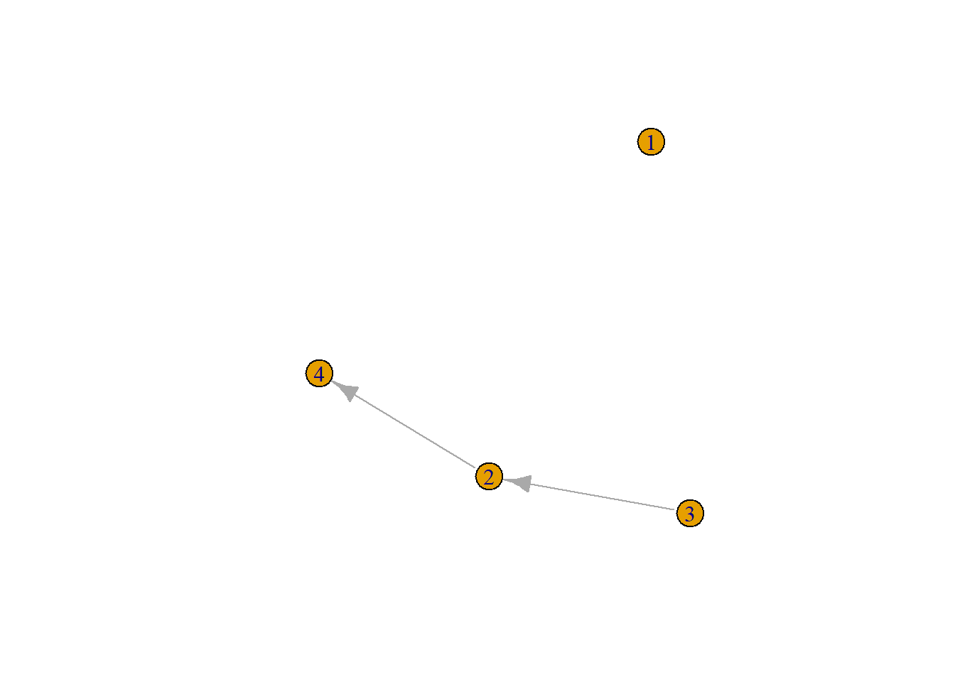
Figure 6.1: small random graph

This is a directed graph, thus node 3 is connected to node 4 (path length 2) but 4 is not connected to 3. What is the average path length? …
It is: 1.33.

The average path length in Smallworld is very low considering the size (105) and density (0.14), it is: 2.13. Since path length excludes disconnected nodes, it does not necessarily tells us something about the ‘degrees of separation’. Let us instead calculate for each path length the proportion of nodes each node can reach and take the average value of that.

To do that, we will make use of the function ego_size in the igraph package. See code chunk below for an example.

mean((ego_size(random_graph, order = 2, mode = "out") - 1)/vcount(random_graph))

#> [1] 0.1875

Thus for the small random graph above, Figure 6.1, if we take a path length of two we find that nodes 1 to 4 node can reach 0, 0.25, 0.5, 0 of all other nodes, respectively. This makes for an average reach of 0.1875.

For Smallworld 2.2 we find the following:

• path length one: 0.13%.
  
• path length two: 0.72%.
  
• path length three: 0.99%.

This brings us to the six-degrees-of-separation phenomenon. This is the observation that for real societies and real worlds 100% of the population would be connected to 100% of the population via 6 other persons (making for a path length of seven). Phrased otherwise, with path length seven, the average reach would be 100%.

The idea that all people are connected through just six degrees of separation is based on Stanley Milgram’s famous ‘The small world problem’ paper (Milgram 1967). Luckily, you don’t need to read the paper. Just watch the movie:

6.1.2 Segregation

There are many ways how to determine the degree of segregation in social networks. See (Bojanowski and Corten 2014). A quite straightforward way is to compare inter- and intra-ethnic group densities (see: the chapter on Network Visualization.

Moran’s I

While inter-/intra group density and for example Coleman’s homophily index describe the extent to which similar people are more likely to be connected. We now take a slightly different angle. We want to know if nodes who are closer to one another in the network are more a like. To which my students respond in unison with:

“Hey, that sounds like some sort of correlation!”

Yup, we need some spatial autocorrelation measure. Let us use Moran’s I for this.
We will start with a calculation of the correlation between the score of actor i and the (mean) score of the alters of i to whom i is connected directly.

Spatial autocorrelation measures are actually quite complex. A lot of build in functions in different packages of R are not very clear on all the defaults. With respect to Moran’s I, its values are actually quite difficult to compare across different spatial/network settings. Results may depend heavily on whether or not you demean your variables of interest, the chosen neighborhood/weight matrix (and hence on distance decay functions and type of standardization of the weight matrix). Anyways, lets get started.

Moran’s I is given by:

\[I= \gamma \Sigma_i\Sigma_jw_{ij}z_iz_j,\]

where \(w_{ij}\) is the weight matrix \(z_i\) and \(z_j\) are the scores in deviations from the mean. And,

\[\gamma= S_0 * m_2 = \Sigma_i\Sigma_jw_{ij} * \frac{\Sigma_iz_i^2}{n},\]

with: \(S_0 = \Sigma_i\Sigma_jw_{ij}\) and \(m_2 = \frac{\Sigma_iz_i^2}{n}\).

Thus \(S_0\) is the sum of the weight matrix and \(m_2\) is an estimate of the variance. For more information see Anselin 1995.

We need two packages, if we not want to define all functions ourselves: sna and ape.¹²

Let us demonstrate the concept on the build-in dataset of RSiena, s50. See also ?s50. For now, we only need to know this data set offers information on friendship ties and alcohol consumption among pupils in a school.

We want to answer the following question:

Are pupils who are close to each other in the network more likely to exhibit similar drinking behavior?

Or phrased otherwise:

Is the network segregated based on drinking behavior?

First use sna. Of course we need to define ‘close’. Let us give alters a weight of 1 if they are part of the 1.0 degree egocentric network and 0 otherwise.

require(RSiena)
library(network)
friend.data.w1 <- s501
friend.data.w2 <- s502
friend.data.w3 <- s503
drink <- s50a
smoke <- s50s

net1 <- network::as.network(friend.data.w1)
net2 <- network::as.network(friend.data.w2)
net3 <- network::as.network(friend.data.w3)

# nacf does not row standardize!
snam1 <- sna::nacf(net1, drink[, 1], type = "moran", neighborhood.type = "out", demean = TRUE)
snam1[2]  #the first order matrix is stored in second list-element

#>         1 
#> 0.4331431

Lets calculate the same thing with ape.

require(ape)
require(sna)
geodistances <- geodist(net1, count.paths = TRUE)
geodistances <- geodistances$gdist

# first define a nb based on distance 1.
weights1 <- geodistances == 1

# this function rowstandardizes by default
ape::Moran.I(drink[, 1], scaled = FALSE, weight = weights1, na.rm = TRUE)

#> $observed
#> [1] 0.486134
#> 
#> $expected
#> [1] -0.02040816
#> 
#> $sd
#> [1] 0.132727
#> 
#> $p.value
#> [1] 0.000135401

Close but not the same value!

Lets use ‘my own’ function and don’t rowstandardize.

fMoran.I <- function(x, weight, scaled = FALSE, na.rm = FALSE, alternative = "two.sided", rowstandardize = TRUE) {
    if (rowstandardize) {
        if (dim(weight)[1] != dim(weight)[2])
            stop("'weight' must be a square matrix")
        n <- length(x)
        if (dim(weight)[1] != n)
            stop("'weight' must have as many rows as observations in 'x'")
        ei <- -1/(n - 1)
        nas <- is.na(x)
        if (any(nas)) {
            if (na.rm) {
                x <- x[!nas]
                n <- length(x)
                weight <- weight[!nas, !nas]
            } else {
                warning("'x' has missing values: maybe you wanted to set na.rm = TRUE?")
                return(list(observed = NA, expected = ei, sd = NA, p.value = NA))
            }
        }
        ROWSUM <- rowSums(weight)
        ROWSUM[ROWSUM == 0] <- 1
        weight <- weight/ROWSUM
        s <- sum(weight)
        m <- mean(x)
        y <- x - m
        cv <- sum(weight * y %o% y)
        v <- sum(y^2)
        obs <- (n/s) * (cv/v)
        if (scaled) {
            i.max <- (n/s) * (sd(rowSums(weight) * y)/sqrt(v/(n - 1)))
            obs <- obs/i.max
        }
        S1 <- 0.5 * sum((weight + t(weight))^2)
        S2 <- sum((apply(weight, 1, sum) + apply(weight, 2, sum))^2)
        s.sq <- s^2
        k <- (sum(y^4)/n)/(v/n)^2
        sdi <- sqrt((n * ((n^2 - 3 * n + 3) * S1 - n * S2 + 3 * s.sq) - k * (n * (n - 1) * S1 - 2 * n *
            S2 + 6 * s.sq))/((n - 1) * (n - 2) * (n - 3) * s.sq) - 1/((n - 1)^2))
        alternative <- match.arg(alternative, c("two.sided", "less", "greater"))
        pv <- pnorm(obs, mean = ei, sd = sdi)
        if (alternative == "two.sided")
            pv <- if (obs <= ei)
                2 * pv else 2 * (1 - pv)
        if (alternative == "greater")
            pv <- 1 - pv
        list(observed = obs, expected = ei, sd = sdi, p.value = pv)
    } else {
        if (dim(weight)[1] != dim(weight)[2])
            stop("'weight' must be a square matrix")
        n <- length(x)
        if (dim(weight)[1] != n)
            stop("'weight' must have as many rows as observations in 'x'")
        ei <- -1/(n - 1)
        nas <- is.na(x)
        if (any(nas)) {
            if (na.rm) {
                x <- x[!nas]
                n <- length(x)
                weight <- weight[!nas, !nas]
            } else {
                warning("'x' has missing values: maybe you wanted to set na.rm = TRUE?")
                return(list(observed = NA, expected = ei, sd = NA, p.value = NA))
            }
        }
        # ROWSUM <- rowSums(weight) ROWSUM[ROWSUM == 0] <- 1 weight <- weight/ROWSUM
        s <- sum(weight)
        m <- mean(x)
        y <- x - m
        cv <- sum(weight * y %o% y)
        v <- sum(y^2)
        obs <- (n/s) * (cv/v)
        if (scaled) {
            i.max <- (n/s) * (sd(rowSums(weight) * y)/sqrt(v/(n - 1)))
            obs <- obs/i.max
        }
        S1 <- 0.5 * sum((weight + t(weight))^2)
        S2 <- sum((apply(weight, 1, sum) + apply(weight, 2, sum))^2)
        s.sq <- s^2
        k <- (sum(y^4)/n)/(v/n)^2
        sdi <- sqrt((n * ((n^2 - 3 * n + 3) * S1 - n * S2 + 3 * s.sq) - k * (n * (n - 1) * S1 - 2 * n *
            S2 + 6 * s.sq))/((n - 1) * (n - 2) * (n - 3) * s.sq) - 1/((n - 1)^2))
        alternative <- match.arg(alternative, c("two.sided", "less", "greater"))
        pv <- pnorm(obs, mean = ei, sd = sdi)
        if (alternative == "two.sided")
            pv <- if (obs <= ei)
                2 * pv else 2 * (1 - pv)
        if (alternative == "greater")
            pv <- 1 - pv
        list(observed = obs, expected = ei, sd = sdi, p.value = pv)
    }


}

fMoran.I(drink[, 1], scaled = FALSE, weight = weights1, na.rm = TRUE, rowstandardize = FALSE)

#> $observed
#> [1] 0.4331431
#> 
#> $expected
#> [1] -0.02040816
#> 
#> $sd
#> [1] 0.1181079
#> 
#> $p.value
#> [1] 0.000122962

Same result as nacf function!

What does rowstandardization mean??

• rowstandardize: We assume that each node i is influenced equally by its neighbourhood regardless on how large it. You could compare this to the average alter effect in RSiena)
  
• not rowstandardize: We assume that each alter j has the same influence on i (if at the same distance). You could compare this to the total alter effect in RSiena.

To not standardize is default in sna::nacf, to standardize is default in apa::Moran.I. This bugs me. I thus made a small adaption to apa::Moran.I and now in the function fMoran.I you can choose if you want to rowstandardize or not.

But…

🎵 🎵
“What you really, really want
I wanna, (ha) I wanna, (ha)
I wanna, (ha) I wanna, (ha)
I wanna really, really, really
Wanna zigazig ah”
🎵 🎵
— Spice Girls - Wannabe

What I really would like to see is a correlation between actor i and all the alters to whom it is connected (direct or indirectly) and where alters at a larger distances (longer shortest path lengths) are weighted less.

• step 1: for each acter i determine the distances (shortest path lengths) to all other nodes in the network.
  
• step 2: based on these distances decide on how we want to weigh. That is, determine a distance decay function.
  
• step 3: decide whether or not we want to row-standardize.

# step 1: calculate distances
geodistances <- geodist(net1, count.paths = TRUE)
geodistances <- geodistances$gdist
# set the distance to yourself as Inf
diag(geodistances) <- Inf


# step 2: define a distance decay function. This one is pretty standard in the spatial
# autocorrelation literature but actually pretty arbitrary.
weights2 <- exp(-geodistances)

# step 3: I dont want to rowstandardize.
fMoran.I(drink[, 1], scaled = FALSE, weight = weights2, na.rm = TRUE, rowstandardize = FALSE)

#> $observed
#> [1] 0.2817188
#> 
#> $expected
#> [1] -0.02040816
#> 
#> $sd
#> [1] 0.07532918
#> 
#> $p.value
#> [1] 6.052458e-05

Conclusion: Yes pupils closer to one another are more a like! And ‘closer’ here means a shorter shortest path length. You also observe that the correlation is lower than we calculated previously. Apparently, we are a like to alters very close by (path length one) and less so (or even dissimilar) to alters further off.

6.2 Random graphs

Now that we know how to count dyad and triad configurations, to calculate network properties and to determine the extent of segregation within networks, the follow-up question is: Is this a lot? Or even: Is this significant? Let try to tackle the latter question. What do we mean with significant? Probably something like: The chance, \(p\), to observe our value for network characteristic (or statistic), \(s^{net}\), is smaller than some arbitrary value, \(\alpha\), would we have randomly picked a network from the general population of networks, \(X\), to which our observed network, \(x^o\) belongs.
This leaves us with just two smaller problems. First, what is this population of networks to which our observed network belongs. Second, what is the distribution of values for network characteristic, \(s^{net}\), in this population?

Let us go back to Smallworld. We stated that in a small world network, despite having a low density and being relatively clustered, the relative average path length is small. What do we mean with relative? Well, in SNA it means that if we would make a random graph, the chance is very low (lower than say 5%) that this graph would have a higher degree of clustering and a shorter average path length.

Let us define the population of graphs to which Smallworld belongs as the graphs that have the same size and density.¹³ In igraph you can generate random graphs with the erdos.renyi.game function.
Let us make 1000 random graphs with size 105 (just as in Smallworld) and with a density of 0.14 (just as in Smallworld). And let us make a histogram of all observed average degree of clustering and path lengths.

require(igraph)
dens <- round(graph.density(smallworld), 2)  #save density of smallworld
trial <- 1000  #set number of trials/sims
trialclus <- triallen <- rep(NA, trial)  #define objects in which you are saving results


for (i in 1:trial) {
    random_graph <- erdos.renyi.game(n = 105, p.or.m = dens, directed = FALSE)  #make the random graph
    triallen[i] <- average.path.length(random_graph, unconnected = TRUE)  #calculate average path length
    trialclus[i] <- transitivity(random_graph, isolates = c("NaN"))  #calculate clustering
}


par(mfrow = c(1, 2))
{
    hist(trialclus, xlim = c(0.1, 0.36), main = "average clustering coefficient", xlab = "", )
    abline(v = transitivity(smallworld, isolates = c("NaN")), col = "red", lwd = 3)
}

{
    hist(triallen, xlim = c(1.9, 2.2), main = "average path length", xlab = "")
    abline(v = average.path.length(smallworld, unconnected = TRUE), col = "red", lwd = 3)
}

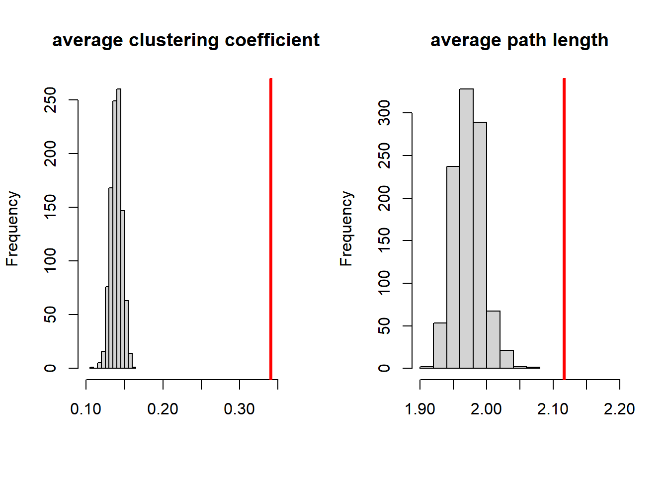
Figure 6.2: Comparing network statistics of Smallworld with random graphs

The values of Smallworld are plotted in red. Smallworld indeed has a very high degree of clustering. Indeed, it is significantly higher than could be expected, because if falls outside more than 99 per cent of the cases of random graphs.
However, we also see that the average path length of Smallworld is significantly higher compared to random graphs. Well, is, or is not, Smallworld a smallworld?
A formal definition of smallworldlyness is:

\[ \sigma = \frac{C/C_r}{L/L_r}, \]

where C is the average clustering of the observed graph and \(C_ r\) is the clustering of the random graph, L is the average shortest path length of the observed graph and \(L_r\) is the average shortest path length of the random graph. With \(\sigma > 1\) the network is said to be a small-world network. The smallworldness of Smallworld is …

…well, try to calculate this for yourself.

C <- transitivity(smallworld, isolates = c("NaN"))
Cr <- mean(trialclus)
L <- average.path.length(smallworld, unconnected = TRUE)
Lr <- mean(triallen)
Sigma <- (C/Cr)/(L/Lr)
print("The smallworldness of Smallworld is:")
Sigma

#> [1] "The smallworldness of Smallworld is:"
#> [1] 2.273717

---

References

Block, Per, Christoph Stadtfeld, and Tom A. B. Snijders. 2019. “Forms of Dependence: Comparing SAOMs and ERGMs from Basic Principles.” Sociological Methods & Research 48 (1): 202–39. https://doi.org/10.1177/0049124116672680.

Bojanowski, Michał, and Rense Corten. 2014. “Measuring Segregation in Social Networks.” Social Networks 39: 14–32.

Milgram, Stanley. 1967. “The Small World Problem.” Psychology Today 2 (1): 60–67.

---

11. With ‘we’ I mean the observers, or the researchers. The social agents do not need to be aware or know all nodes and ties.↩︎

12. I quite frequently need to calculate Moran’s I and related statistics in my work/hobby. I commonly use the functions in the R package spdep.↩︎

13. You could also set an additional filter and only compare graphs which also have the same degree distribution as the actual observed graph (Smallworld in the example).↩︎